| Res.Df | RSS | Df | Sum of Sq | F | Pr(>F) |
|---|---|---|---|---|---|
| 25 | 0 | NA | NA | NA | NA |
| 24 | 0 | 1 | 0 | 2.285 | 0.144 |
Model Evaluation
Nested Models
Last class:
Goodness of fit
RSS, ESS, TSS
the coefficient of determination, \(R^2\)
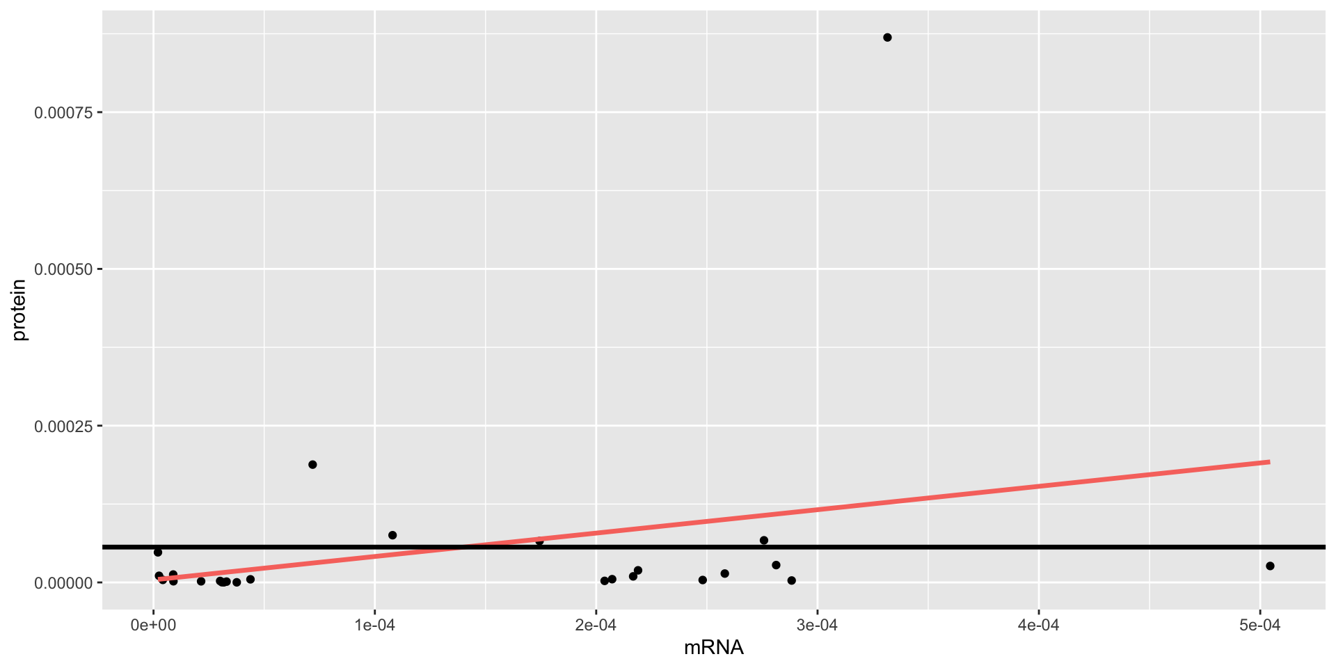
we introduced a new case study from Biology aiming to study the relation between mRNA and protein levels
we evaluated the goodness of fit of SLR and MLR for the data and found a poor fit of the proposed model for most genes
Evaluation metrics
Scroll down to see full content
Many metrics used to evaluate LR measure how far \(y\) is from \(\hat{y}\):
- Residuals Sum of Squares: RSS = \(\sum_{i=1}^n(y_i - \hat{y}_i)^2\)
sum of the squared residuals, small is good
- Residuals Standard Error: RSE = \(\sqrt{\frac{1}{n-p-1} \text{RSS}}\)
gives an idea of the size of the irreducible error, very similar to the RSS, small is good
- Mean Squared Error: MSE = \(\frac{1}{n}\sum_{i=1}^n(y_i - \hat{y}_i)^2\)
mean of the squared residuals, small is good. Usually computed on both the training and the test sets.
Coefficient of Determination
Scroll down to see full content
All the measures listed above are absolute measures
It is not easy to judge if these are small enough. Important relative measures:
- Coefficient of Determination, \(R^2 = 1 - \frac{RSS}{TSS}\)
it also compares \(y\) vs \(\hat{y}\) using the RSS but relative to the TSS (sum of the squared residuals of the intercept-only model)
it is a common measure of goodness of fit: how well does the model fit the training data?
it doesn’t have a known distribution so you can’t use it to test a statistical hypothesis
it increases with the size of the model so it is not useful to compare models of different sizes
Adjusted \(R^2\)
\(\text{adj}R^2 = 1 - \frac{RSS/(n-p-1)}{TSS/(n-1)}\)
it is a common measure of goodness of fit: how well does the model fit the training data?
penalizes the RSS by the size of the model so it can be used to compare models of different sizes
Today
Comparing nested models
F-test for goodness of fit
a more general F-test
The F-test
Although the \(R^2\) is a widely used measure to evalute goodness of fit, it is not a formal statistical test.
Test: is the full model significantly different from an intercept-only model?
The intercept-only model does not include any covariate, thus the estimated coefficient is given by the mean of the response, \(\bar{Y}\), in our case the average protein value
The test hypotheses
model reduced: \(Y_i=\beta_0 + \varepsilon_i\)
model full: \(Y_i=\beta_0 + \beta_1 X_{i1} + \ldots + \beta_p X_{ip} + \varepsilon_i\)
We are simulataneously testing if many coefficients are zero!!
\[H_0: \beta_{1} = \beta_{2} = \ldots = \beta_{p} = 0\]
against
\[H_1: \text{at least one } \beta_j \neq 0 \text{ (for } j = 1, 2, \dots, p \text{)}\]
The \(F\)-statistic
\[\frac{(RSS_{reduced}-RSS_{full})/p}{RSS_{full}/(n-p-1)} \sim \mathcal{F}_{p, n-p-1}\]
\(RSS_{reduced}\) is the RSS of the reduced model
\(RSS_{full}\) is the RSS of the full model
\(p\) is the number of covariates in the full model (excluding the intercept), number of parameters tested
Don’t worry, R computes this statistic for you!!
The \(F\)-test in R
There are 2 functions in R that we can use to perfor this test:
glance(model_full)anova(model_reduced, model_full)
With
glance(), the reduced model is always the intercept-only model
With
anova(), you can compare the full against any reduced model
Back to the case study
The test for model.2
model reduced: \(\text{prot}_i=\beta_0 + \varepsilon_i\)
model.2 full: \(\text{prot}_i=\beta_0 + \beta_1 \text{mrna}_i + \varepsilon_i\)
We are simulataneously testing if many coefficients are zero!!
\[H_0: \beta_{1} = 0\]
\[H_1: \beta_1 \neq 0\]
Note that these are the same hypotheses tested by
lm!!
ANOVA
GLANCE
| r.squared | adj.r.squared | sigma | statistic | p.value | df | logLik | AIC | BIC | deviance | df.residual | nobs |
|---|---|---|---|---|---|---|---|---|---|---|---|
| 0.087 | 0.049 | 0 | 2.285 | 0.144 | 1 | 190.382 | -374.764 | -370.99 | 0 | 24 | 26 |
lm-tidy
| term | estimate | std.error | statistic | p.value |
|---|---|---|---|---|
| (Intercept) | 0.000 | 0.000 | 0.086 | 0.932 |
| mrna | 0.373 | 0.247 | 1.512 | 0.144 |
\(t\)-test vs \(F\)-test
Scroll down to see full content
\(t\)-test
lm() computes \(t\)-tests to evaluate the contribution of each variables to explain a response with possibly other variables included in the model!!
\[H_0: \beta_j = 0, \text{ versus } H_1: \beta_j \neq 0\]
\(H_0\) contains only one coefficient, even if the model has more
The results of the \(t\)-tests evaluate the contribution of each variable (separately) to explain the variation observed in the response
\(F\)-test
glance() computes an \(F\)-test to evaluate the contribution of all variables to explain a response (all vs nothing)!!
\[H_0: \beta_1 = \beta_2 = \ldots = \beta_p = 0, \text{ versus } H_1: \text{at least one } \beta_j \neq 0\]
\(H_0\) contains all coefficient (except the intercept)
Special case: \(p=1\)
If there is only covariate in the full model, the hypotheses are the same!
It can be shown that the \(F\)-test (by
glance) is equivalent to the \(t\)-test (bylm): \(F=t^2\) and equal \(p\)-values
Both tests (\(F\) and \(t\)) are based on Normality assumptions or approximate Normality distribution given by large sample theory
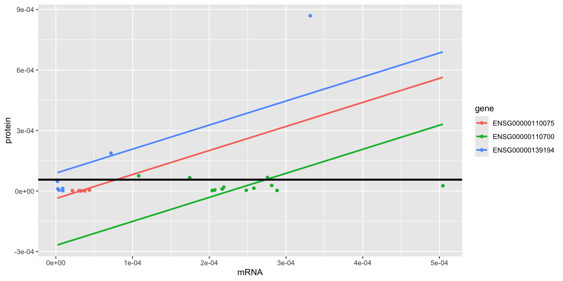
The test for model.4
model reduced: \(\text{prot}_i=\beta_0 + \varepsilon_i\)
model.4 full: \(\text{prot}_t=\beta_0 + \beta_1 \text{mrna}_{t} + \beta_2 \text{gene2}_{t} + \beta_3 \text{gene3}_{t} + \varepsilon_t\)
We are simulataneously testing if many coefficients are zero!!
\[H_0: \beta_{1} = \beta_{2} = \beta_{3} = 0\]
\[H_1: \text{at least one } \beta_j \neq 0, \text{ for } j = 1,2, 3\]
These are not the same hypotheses tested by
lm!!
ANOVA
| Res.Df | RSS | Df | Sum of Sq | F | Pr(>F) |
|---|---|---|---|---|---|
| 25 | 0 | NA | NA | NA | NA |
| 22 | 0 | 3 | 0 | 7.941 | 0.001 |
GLANCE
| r.squared | adj.r.squared | sigma | statistic | p.value | df | logLik | AIC | BIC |
|---|---|---|---|---|---|---|---|---|
| 0.52 | 0.454 | 0 | 7.941 | 0.001 | 3 | 198.738 | -387.476 | -381.186 |
lm-tidy
| term | estimate | std.error | statistic | p.value |
|---|---|---|---|---|
| (Intercept) | 0.000 | 0.00 | -0.770 | 0.450 |
| mrna | 1.192 | 0.29 | 4.112 | 0.000 |
| geneENSG00000110700 | 0.000 | 0.00 | -2.681 | 0.014 |
| geneENSG00000139194 | 0.000 | 0.00 | 1.859 | 0.076 |
Interpretation:
For these 3 genes, the \(p\)-value of the \(F\)-test is less than 0.05.
There is enough evidence to reject the null hypothesis.
The estimated additive model (common slope and different intercepts) is significantly better than the average protein value from the intercept-only model.
IMPORTANT: this doesn’t mean that we can predict protein from mRNA!
There is another variable in the model gene that may be as (or more) important as mRNA
More general
The \(F\)-test can be used to compare any pair of nested models
LR with \(q+1\) coefficients
- model reduced: \(Y_i=\beta_0 + \beta_1 X_{i1} + \ldots + \beta_q X_{iq} + \varepsilon_i\)
LR with \(p+1\) coefficients, \(k\) additional explanatory variables
- model full: \(Y_i=\beta_0 + \beta_1 X_{i1} + \ldots + \beta_q X_{iq} + \ldots + \beta_p X_{ip} + \varepsilon_i\)
Case example
For example:
- model.2 reduced:
lm(prot ~ mrna)
\[\text{prot}_i=\beta_0 + \beta_1 \text{mrna}_{t} + \varepsilon_i\]
- model.4 full:
lm(prot ~ mrna + gene)
\[\text{prot}_t=\beta_0 + \beta_1 \text{mrna}_{t} + \beta_2 \text{gene2}_{t} + \beta_3 \text{gene3}_{t} + \varepsilon_t\]
The test hypotheses
We are simulataneously testing if many parameters (all the additional ones) are zero!!
\[H_0: \beta_{q+1} = \beta_{q+2} = \ldots = \beta_{p} = 0\]
against
\[H_1: \text{at least one } \beta_j \neq 0 \text{ (for } j = q+1, q+2, \dots, p \text{)}\]
The F-statistic
\[\frac{(RSS_{reduced}-RSS_{full})/k}{RSS_{full}/(n-p-1)} \sim \mathcal{F}_{k, n-p-1}\]
\(RSS_{reduced}\) is the RSS of the reduced model
\(RSS_{full}\) is the RSS of the full model
\(k\) is the number of parameters tested (#full - #reduced)
\(p\) is the number of covariates in the full model (excluding the intercept)
Don’t worry, R computes this statistic for you!!
The \(F\)-test in R
For any reduced model, other than the intercept-only:
anova(model_reduced, model_full)
With
glance()the reduced model is always the intercept-only model
In our example
Scroll down to see full content
model.2 reduced:
lm(prot ~ mrna), \(\text{prot}_i=\beta_0 + \beta_1 \text{mrna}_{t} + \varepsilon_i\)model.4 full:
lm(prot ~ mrna + gene), \(\text{prot}_t=\beta_0 + \beta_1 \text{mrna}_{t} + \beta_2 \text{gene2}_{t} + \beta_3 \text{gene3}_{t} + \varepsilon_t\)
\[H_0: \beta_{2} = \beta_{3} = 0\]
\[H_1: \text{at least one } \beta_j \neq 0, \text{ for } j = 2, 3\]
Model Selection
Do we need all the available predictors in the model?
Some datasets contain many variables but not all are relevant
you may want to identify the most relevant variables to build a model
People use the \(F\)-test and even the \(t\)-tests to select significant variables and then re-fit the model using the selected variables
Warning
Caution: the data is used over (and over) again to select so inference results are not longer valid. Post-inference problem
Summary
The \(R^2\), coefficient of determination, can be used to compared the sum of squares of the residuals of the fitted model with that of the intercept-only model
The \(R^2\) is usually interpreted as the part of the variation in the response explained by the model
Many definitions and interpretations of the \(R^2\) are for LS estimators of LR containing an intercept
The \(R^2\) can not be used to compare models of different sizes since bigger models always have larger \(R^2\).
Instead, the adj\(R^2\) can be computed to take into account the sizes of the models.
The \(R^2\) is not a test and it does not provide a probabilistic result and it’s distribution is unknown!
Instead, we can use an \(F\) test, using
anova(), to compare nested modelstests the simultaneous contribution of additional coefficients of the full model (not in the reduced model)
in particular, we can use it to assess the significance of the full model over the intercept-only model (using
glance()oranova())
These \(F\) tests can be used to select among nested models.
Warning
Caution: you may need to partition the data to avoid a post-inference problem (more coming in week 10)
© 2025 Gabriela Cohen Freue – Material Licensed under CC By-SA 4.0