Model Evaluation

Goodness of Fit

Part 1: Model Estimation and Tests

  • Linear regression: continuous response

  • Logistic regression: binary response

  • Poisson regression: count response

  • Diagnostics of assumptions

This week: Model Evaluation

Photo by Siora Photography on Unsplash

Does the model fit the data well? Do we need more/less variables in the model?

This week

We will evaluate different linear models estimated by least squares (LS)

Today: Goodness of fit

  • the coefficient of determination, \(R^2\)

  • other evaluation metrics

Next class: comparing nested models

  • \(F\)-test to compare our model against an intercept-only model

  • a more general F-test to compare nested models

Case Study: protein vs mRNA

We will work with a new case study from Biology aiming to study the relation between mRNA and protein levels

  • the Central Dogma of Biology: protein levels should be highly related to mRNA levels

  • however, most experimental data found weak associations between these features

Can we predict protein from mRNA levels??

An ambitious result

An ambitious claim

Scroll down to see full content

In 2014, Wilhelm et al. proposed a method to predict protein from mRNA levels and claimed:

[…] it now becomes possible to predict protein abundance in any given tissue with good accuracy from the measured mRNA

For each gene \(g\) the predicted protein level in the \(t\)-th tissue is given by

\[\hat{\text{prot}}_{t} = \hat{r}_g * \text{mrna}_{t}\]

where, \(\hat{r}_g\) is the median of all the prot/mrna ratios of gene g

The subscript \(t\) is to identify each tissue.

The subscript \(g\) is to emphasize that the slope is gene-specific.

Models (examples for 3 genes)

Scroll down to see full content

  • model.1:

\[\text{prot}_t=\beta_0 + \varepsilon_t\]

  • model.2:

\[\text{prot}_t=\beta_0 + \beta_1 \text{mrna}_{t} + \varepsilon_t\]

  • model.3:

\[\text{prot}_t=\beta_0 + \beta_2 \text{gene2}_{t} + \beta_3 \text{gene3}_{t} + \varepsilon_t\]

  • model.4:

\[\text{prot}_t=\beta_0 + \beta_1 \text{mrna}_{t} + \beta_2 \text{gene2}_{t} + \beta_3 \text{gene3}_{t} + \varepsilon_t\]

  • model.5:

\[\text{prot}_t=\beta_0 + \beta_1 \text{mrna}_{t} + \beta_2 \text{gene2}_{t} + \beta_3 \text{gene3}_{t} + \beta_4 \text{gene2}_{t}\text{mrna}_{t} + \beta_5 \text{gene3}_{t}\text{mrna}_{t} + \varepsilon_t\]

Wilhelm et al.: “translation rate is a fundamental, encoded (constant) characteristic of a transcript [gene]

model.2: SLR

set.seed(561)
dat_3genes <- dat_bio  %>% 
         subset(gene %in% sample(gene,3))

model2 <- lm(prot~mrna, data=dat_3genes)
tidy(model2)
# A tibble: 2 × 5
  term          estimate std.error statistic p.value
  <chr>            <dbl>     <dbl>     <dbl>   <dbl>
1 (Intercept) 0.00000409 0.0000475    0.0860   0.932
2 mrna        0.373      0.247        1.51     0.144

Prediction and residuals

The predicted values

The blue dot, \(\hat{Y}\) in the line, is the predicted protein level for a given amount of mRNA in this gene.

\[\hat{y}_i = \hat{\beta}_0 + \hat{\beta}_1 \; x_{i}\]

we put a “hat” on \(y\) to indicate that it’s a predicted value using the estimated regression

NOTE: there’s no error term in the predicted model!

Predicted values

Scroll down to see full content

  • They are random variables since they are functions of the estimated coefficients

we can estimate their standard error and CI!! (coming next class!)

  • In R output all predicted values are stored in the column .fitted.

In our case:

\[ \hat{\text{prot}}_{t} = 4.18 \times 10^{-6} + 0.37 \text{ mrna}_{t}\]

The residuals

Scroll down to see full content

The residual is the difference between the predicted and the observed value of the response

In R output all residuals are stored in the column .resid.

\[ \text{res}_i = y_{i}-\hat{y}_{i}\]

Note that:

\[\varepsilon_i \ne \text{res}_i\]

The residuals are the prediction errors.

In our case:

\[ \text{res}_t=\text{prot}_{t}-\hat{\text{prot}}_{t}\]

Goodness of fit

Is our model better than “nothing”?

Scroll down to see full content

  • The best predictor of the response \(Y\) is \(E[Y]\) which we can estimate with the sample mean of \(Y\)

  • Given the (additional) information in \(\mathbf{X}\), the best predictor is \(E[Y|\mathbf{X}]\)

“nothing” means no explanatory variables, intercept-only model, aka null model

So, an important question is:

Is our linear regression better than just using \(E[Y]\) to predict??

Statistically, we want to compare our prediction \(\hat{Y}\) (an estimate of \(E[Y|\mathbf{X}]\)) with \(\bar{Y}\) (an estimate of \(E[Y]\))

Comparing predictions

Explained Sum of Squares: \(ESS=\sum_{i=1}^n(\hat{y}_i-\bar{y})^2\)

  • \(\hat{y}_i\) predicts \(y_i\) using the LR

  • \(\bar{y}\) predicts \(y_i\) without a model.

If our model is better than nothing, this should be large!!

The ESS measures how much variation in the data is explained by the additional information given by the LR

Residual Sum of Squares: \(RSS=\sum_{i=1}^n(y_i - \hat{y}_i)^2\)

  • this is the sum of the squares of the residuals from the fitted model

  • our estimated parameters minimize these distances!!

Total Sum of Squares: \(TSS=\sum_{i=1}^n(y_i-\bar{y})^2\)

  • this is the sum of the squares of the residuals from the null (intercept-only, no explanatory variables) model

  • when properly scaled, it is the sample variance of \(Y\) which estimates the population variance of \(Y\)

Sum of squares decomposition

If parameters are estimated using LS and the LR has an intercept, TSS=ESS + RSS

\[\sum_{i=1}^n(y_i-\bar{y})^2 = \sum_{i=1}^n(\hat{y}_i-\bar{y})^2 + \sum_{i=1}^n(y_i - \hat{y}_i)^2\]

The coefficient of determination

Scroll down to see full content

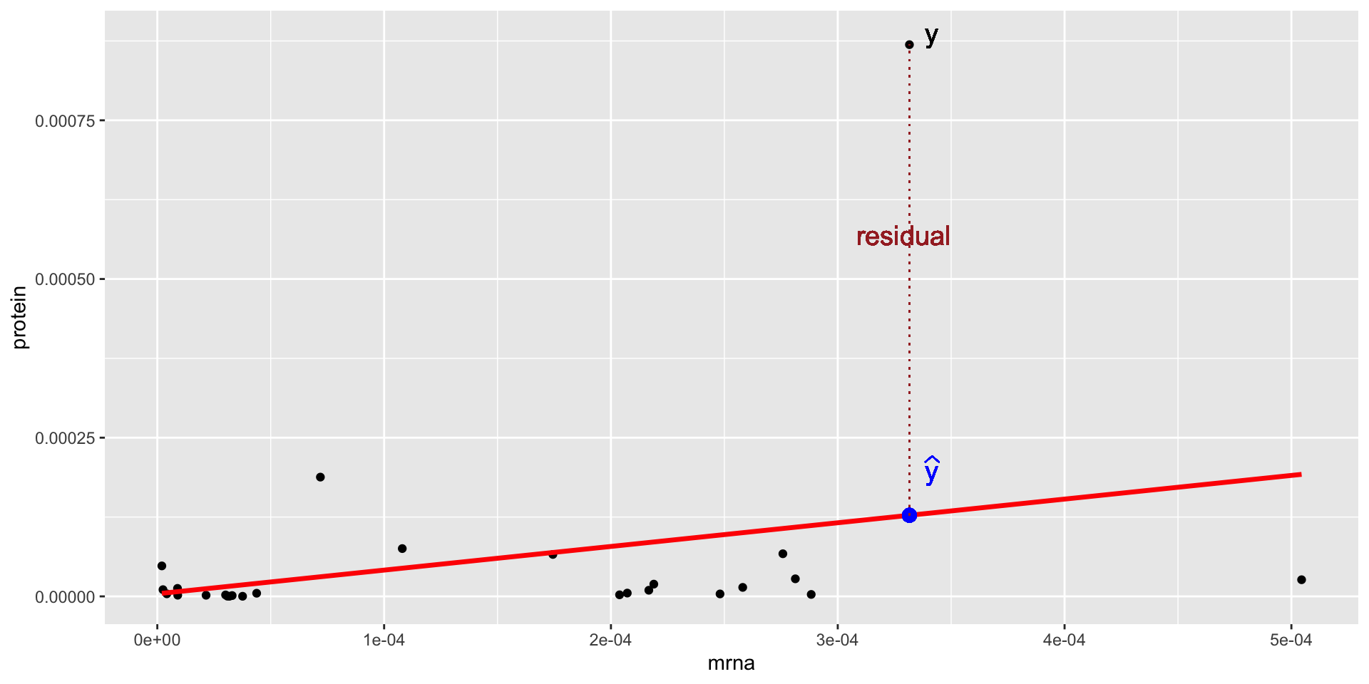
If our model provides a good fit, we expect the TSS (residuals from the null model, in red) to be much larger than the RSS (residuals from the fitted model, which we minimized by LS, in blue)!!

Picture from Wikipedia

Using the decomposition above and dividing by TSS:

\[1=\frac{\text{ESS}}{\text{TSS}} + \frac{\text{RSS}}{\text{TSS}}\]

The Coefficient of determination was first defined as:

\[R^2=1 - \frac{\text{RSS}}{\text{TSS}}\]

For a LR with an intercept and estimated by LS it is equivalent to

\[R^2=\frac{\text{ESS}}{\text{TSS}}\]

Interpretations

For a LR with an intercept and estimated by LS, the coefficient of determination:

  • measures the gain in predicting the response using the LM instead of the response sample mean, relative to the total variation in the response.

  • is also interpreted as the proportion of variance of the response (TSS) explained by the model (ESS)

  • is between 0 and 1 since we expect TSS to be much larger than RSS (thus their ratio is smaller than 1)

1.3 Computing in R

Don’t worry, R computes this statistic for you!!

For the full model

glance(model2)
# A tibble: 1 × 12
  r.squared adj.r.squared    sigma statistic p.value    df logLik   AIC   BIC
      <dbl>         <dbl>    <dbl>     <dbl>   <dbl> <dbl>  <dbl> <dbl> <dbl>
1    0.0869        0.0489 0.000166      2.29   0.144     1   190. -375. -371.
# ℹ 3 more variables: deviance <dbl>, df.residual <int>, nobs <int>

  • For the 3 genes randomly selected in this example, only 9% of the total variation in protein levels is explained by mrna!!

  • The coefficient of determination equals the square of the coefficient of multiple correlation

you probably noticed this in the SLR: \(r^2=R^2\)

in fact, the coefficient of determination was first introduced this way in 1921!

For gene-specific models

Let’s look at each gene separately

                gene values.av tissue         prot      mrna
1308 ENSG00000110075         7 uterus           NA 0.0000337
1324 ENSG00000110700        12 uterus 2.767271e-05 0.0002813
2572 ENSG00000139194         7 uterus 1.871157e-06 0.0000090
6132 ENSG00000110075         7 kidney           NA 0.0000269
6148 ENSG00000110700        12 kidney 6.606698e-05 0.0001744
7396 ENSG00000139194         7 kidney 8.691741e-04 0.0003316
dat_3genes  %>% group_by(gene)  %>% 
                do(glance(lm(prot ~ mrna, data = .)))
# A tibble: 3 × 13
# Groups:   gene [3]
  gene      r.squared adj.r.squared   sigma statistic p.value    df logLik   AIC
  <fct>         <dbl>         <dbl>   <dbl>     <dbl>   <dbl> <dbl>  <dbl> <dbl>
1 ENSG0000…    0.179         0.0142 1.69e-6     1.09  3.45e-1     1   84.3 -163.
2 ENSG0000…    0.0609       -0.0330 2.77e-5     0.648 4.39e-1     1  110.  -214.
3 ENSG0000…    0.996         0.995  2.22e-5  1229.    3.55e-7     1   66.2 -126.
# ℹ 4 more variables: BIC <dbl>, deviance <dbl>, df.residual <int>, nobs <int>

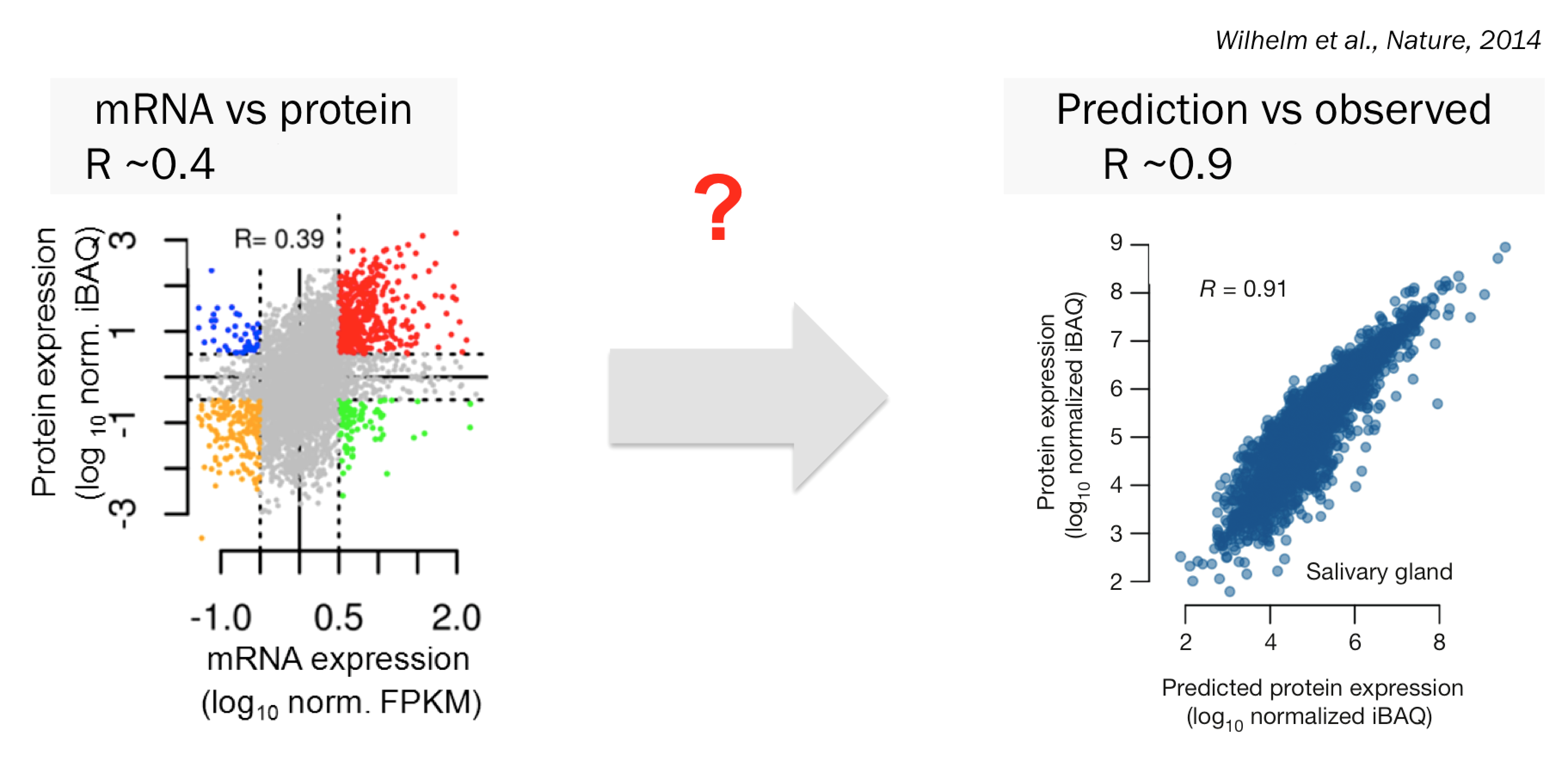
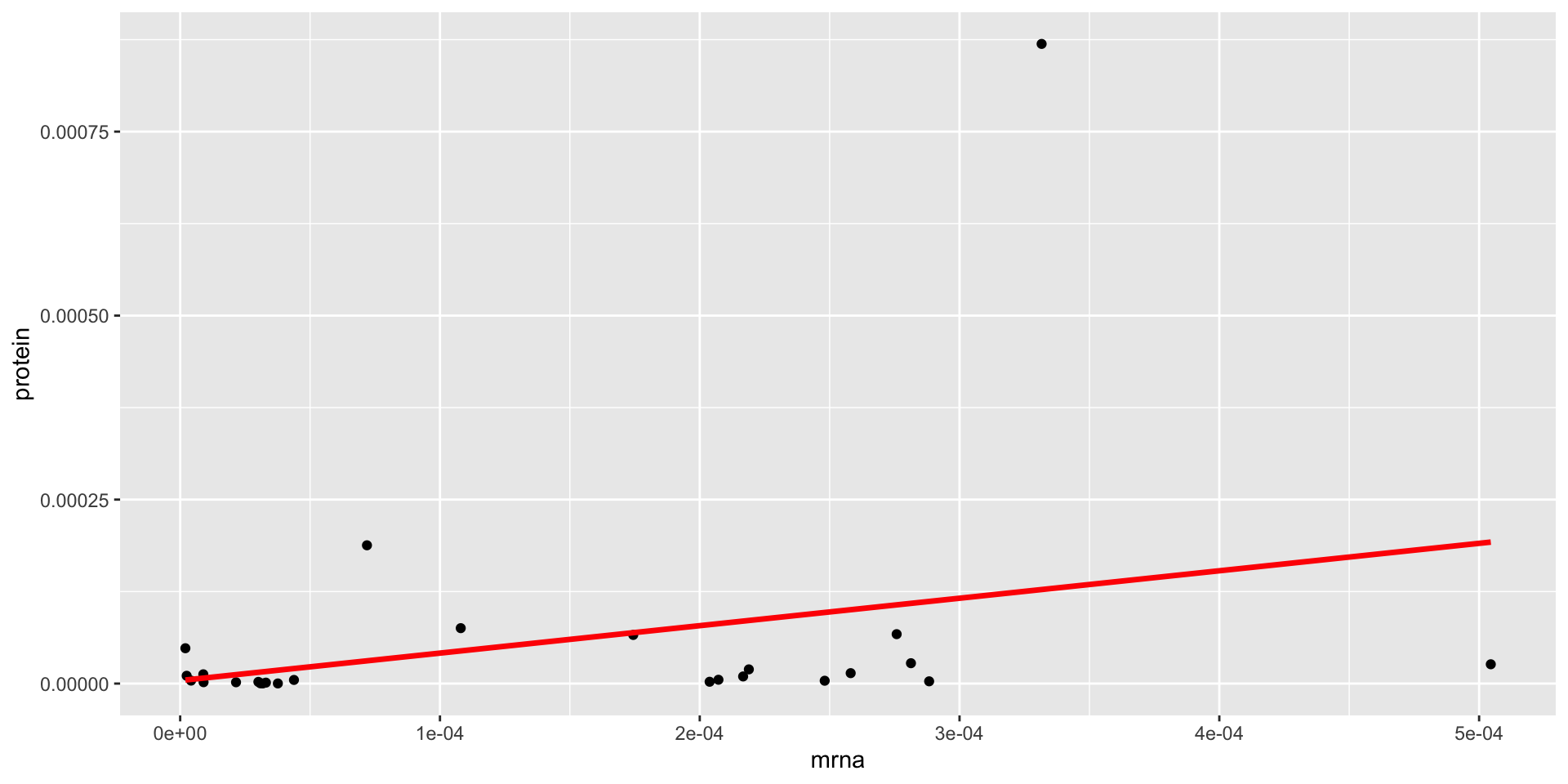
For the majority of the genes, the SLR does not fit the data well

Is the \(R^2\) useful??

Scroll down to see full content

When we use LS, we get an \(R^2=0.56\), is this value large??

  • The \(R^2\) can be used to compare the size of the residuals of the fitted model with those of the null

  • The \(R^2\) can’t be used to test any hypothesis to answer this question since its distribution is unknown

  • The \(R^2\) is computed based on in-sample observations

  • The \(R^2\) does not provide a sense of how good is our model in predicting out-of-sample cases (aka test set)!!

  • Note that \(R^2\) computed as \(R^2 = 1 - \frac{\text{RSS}}{\text{TSS}}\) ranges between 0 and 1 if the LR model has an intercept and is estimated by LS!!

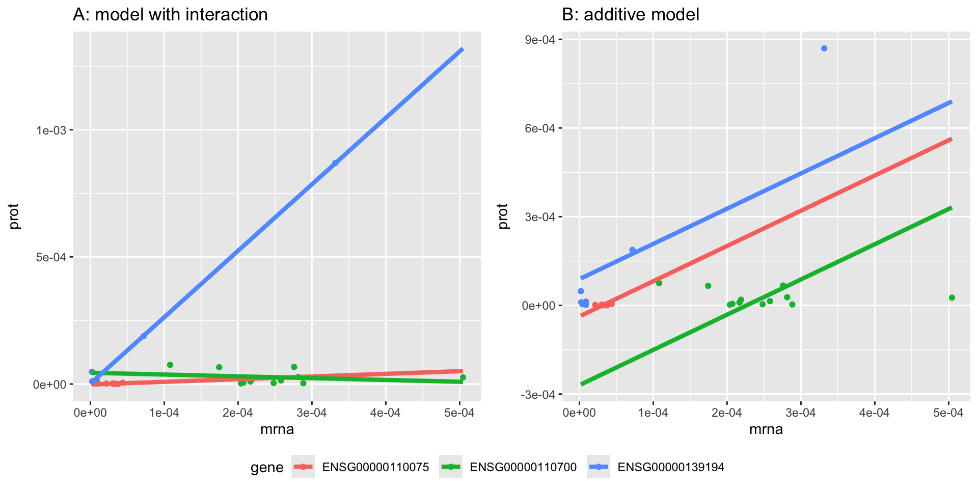
  • The \(R^2\) increases as new variables are added to the model, regardless of their relevance!! Thus, it can’t be used to compare nested models

Model Evaluation via Adjusted \(R^2\)

Scroll down to see full content

The \(R^2\) increases as more input variables are added to the model since the \(\text{RSS} = \sum_{i = 1}^n(y_i - \hat{y}_i)^2\) decreases as more input variables are included in the model.


To overcome this issue with \(R^2\), we can obtain an adjusted \(R^2\) as follows:

\[ \text{adjusted } R^2 = 1- \frac{\text{RSS}/(n - p -1)}{\text{TSS}/(n - 1)},\]

where

  • \(p\) is the number of covariates in the model (excluding the intercept)
  • \(n\) is our sample size to estimate the model

This adjusted coefficient of determination penalizes \(\text{RSS}\) with \(n - p - 1\). Hence, even if the \(\text{RSS}\) decreases, we divide it by \(n - p -1\) to compensate for the model’s size.

Other evaluation metrics

Scroll down to see full content

Other related metrics used to evaluate LR which measure how far \(Y\) is from \(\hat{Y}\) are:

Residuals Standard Error: RSE = \(\sqrt{\frac{1}{n-p - 1} \text{RSS}}\)

called sigma in glance() output

  • The RSE estimates the standard deviation of the error term \(\varepsilon\) (the RSS is divided by the appropriate degrees of freedom to give a “good” estimate of \(\sigma = \sqrt{Var(\varepsilon)}\))


  • The RSE is a measure based on training data to evaluate the fit of the model (for inference) and needed to estimate the standard errors of \(\hat{\beta}_j\) in classical theory!


  • The RSE gives an idea of the size of the irreducible error, very similar to the RSS, small is good

Mean Squared Error: MSE = \(\frac{1}{n}\sum_{i=1}^n(y_i - \hat{y}_i)^2\)

  • Training MSE: if we use the original sample \(y_1, \ldots, y_n\) and their predicted values (formula above). It can be easily obtained from .resid column in augment() output


  • Testing MSE: can be computed on new data \(y_{\text{new}}\) and their predicted values (formula above) to evaluate out-of-sample prediction performance

iClicker questions

Question 1: model.1

Which of the following codes would you use to estimate the model below:

\[\text{prot}_t = \beta_0 + \varepsilon_t\]

  • A dat_3genes %>% lm(prot ~ ., data = .) %>% tidy()

  • B dat_3genes %>% group_by(gene) %>% do(model=tidy(lm(prot ~ 1, data = .))) %>% pull()

  • C dat_3genes %>% lm(prot ~ 1, data = .) %>% tidy()

  • D dat_3genes %>% lm(prot ~ mrna , data = .) %>% tidy()

Question 2: model.2

Which of the following codes would you use to estimate the model below:

\[\text{prot}_t = \beta_0 + \beta_1 \times \text{mrna}_t + \varepsilon_t\]

  • A dat_3genes %>% lm(prot ~ mrna, data = .) %>% tidy()

  • B dat_3genes %>% group_by(gene) %>% do(model=tidy(lm(prot ~ mrna, data = .))) %>% pull()

  • C dat_3genes %>% lm(prot ~ mrna + gene, data = .) %>% tidy()

Question 3: model.3

Which of the following codes would you use to estimate the model below:

\[\text{prot}_t = \beta_0 + \beta_1 \times \text{gene2}_t + \beta_2 \times \text{gene3}_t +\varepsilon_t\]

  • A dat_3genes %>% lm(prot ~ ., data = .) %>% tidy()

  • B dat_3genes %>% group_by(gene) %>% do(model=tidy(lm(prot ~ 1, data = .))) %>% pull()

  • C dat_3genes %>% lm(prot ~ 1, data = .) %>% tidy()

  • D dat_3genes %>% lm(prot ~ gene , data = .) %>% tidy()

Question 4: model.4

Which of the following plots represent the following model in:

\[\text{prot}_t = \beta_0 + \beta_1 \times \text{mrna}_t + \beta_2 \times \text{gene2}_t + \beta_3 \times \text{gene3}_t + \varepsilon_t\]