Logistic Regression

from a mathematical perspective

Last class

Logistic Regression

Logistic regression is a powerful statistical method used for modelling binary responses.

Unlike linear regression, which predicts continuous values, logistic regression predicts the probability of a binary event occurring (e.g., success/failure, yes/no, or true/false).
Logistic regression not only provides interpretable coefficients but also allows for effective classification tool.

In this lecture

A mathematical exploration of the model

Linear component
Probability, odds and log odds
Odds ratios

Interpretation of coefficients

for simplicity, only one input variable is used in this lecture, but everything holds for many variables

Logistic Regression

In MLR we model the conditional expectation of the response as a linear model:

\[E(Y_i|X_i) = \beta_0 + \beta_1X_i\]

Range problem: for a binary response the conditional expectation is a probability (i.e., probability of success), thus a number between 0 and 1.

For a binary response \(Y_i\),

\[E(Y_i|X_i) = P(\left.Y_{i} = 1 \right| X_{i}) = p_i \]

Logistic curve

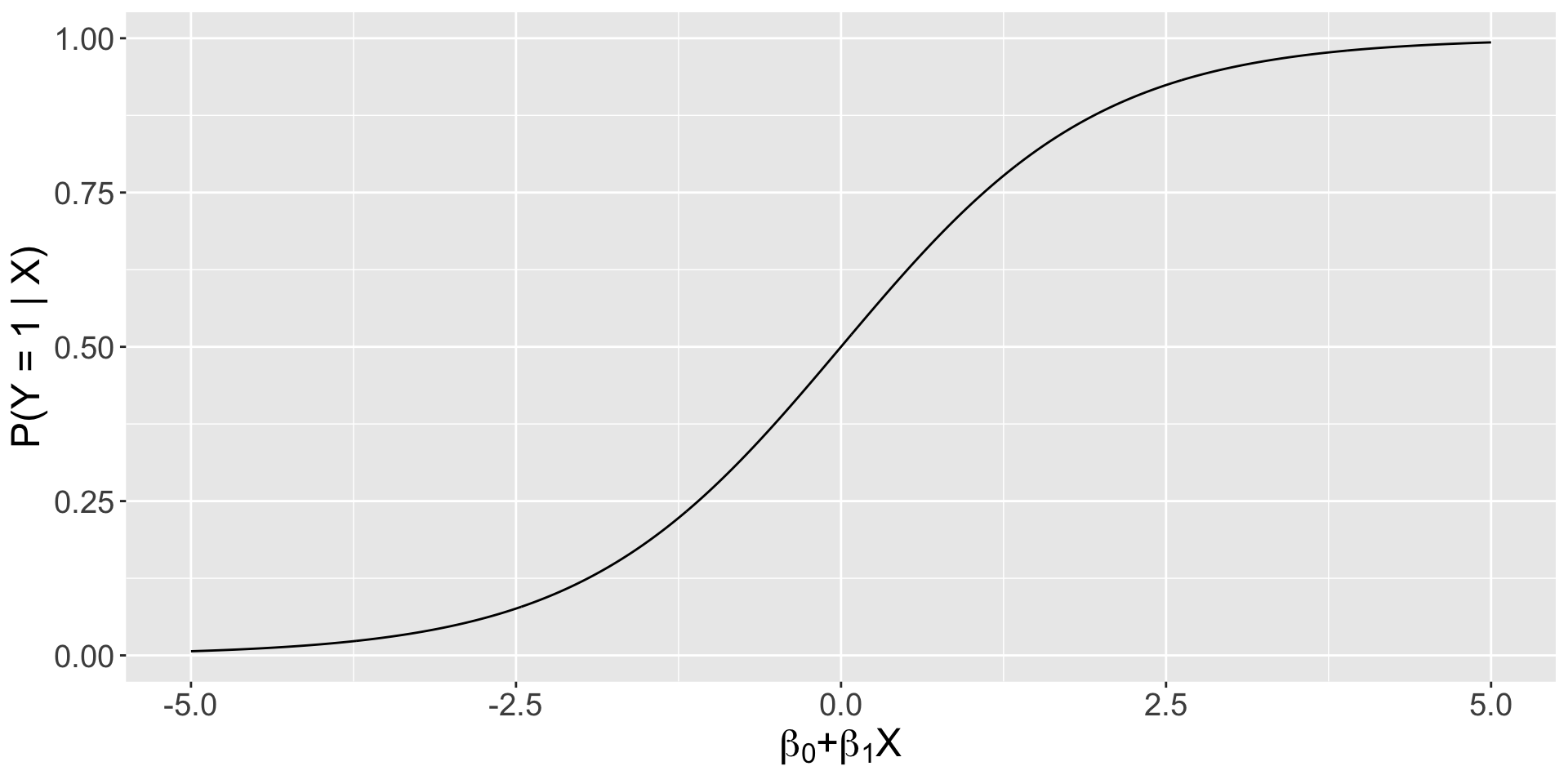
So, instead of a “line” to model the conditional expectation, we need a function of the line with values between 0 and 1! In this course, we will use the logistic function:

\[E(Y_i|X_i) = P(\left.Y_{i} = 1 \right| X_{i}) = p_i = \frac{e^{\beta_0 + \beta_1X_i}}{1+e^{\beta_0 + \beta_1X_i}}\]

Note that \(e^{\beta_0 + \beta_1X_i}\) and \((1+e^{\beta_0 + \beta_1X_i})\) are always positive, and the denominator is larger than the numerator. Thus, this ratio is always between 0 and 1!!

there are many other functions with a range \([0,1]\)!

Plot of the logistic function

Mathematical equivalences

For simplicity, let \(L\) be the linear component: \(L=\beta_0 + \beta_1X_i\)

\[\begin{aligned} p_i &= \frac{e^{L}}{1+e^{L}}\\ (1+e^{L})\times p_i &=e^{L}\\ p_i+p_ie^{L} &=e^{L}\\ p_i &=e^{L}-p_ie^{L}\\ p_i &=e^{L}(1-p_i)\\ \frac{p_i}{1 - p_i} &= e^{L} \end{aligned}\]

Probability vs odds

We showed that we can use the Logistic regression to model either the (conditional) probability or the odds of success!

\[E(Y_i|X_i) = P(\left.Y_{i} = 1 \right| X_{i}) = p_i = \frac{e^{\beta_0 + \beta_1X_i}}{1+e^{\beta_0 + \beta_1X_i}} \qquad [\text{probabilities}]\]

\[ \frac{P(\left.Y_{i} = 1 \right| X_{i})}{1-P(\left.Y_{i} = 1 \right| X_{i})} = \underbrace{\frac{p_i}{1-p_i}}_{\textbf{odds of success}} = e^{\beta_0 + \beta_1 X_{i}} \qquad [\text{odds}] \]

Note that none of these models are linear!

Logistic: a generalized linear model

… but we are very close to a linear model.

Taking log of the last equation we get:

\[ \log\left(\frac{P(\left.Y_{i} = 1 \right| X_{i})}{1-P(\left.Y_{i} = 1 \right| X_{i})}\right) = \underbrace{\log\left(\frac{p_i}{1-p_i}\right)}_{\textbf{log-odds or logit}} = \beta_0 + \beta_1 X_{i}\quad [\text{log odds}] \]

The logit is linear in \(X\)! so the logistic regression belongs to the family of generalized linear models.

Understanding odds

A natural way of interpreting the coefficients of a logistic regression is based on odds. Let’s take a closer look at this quatity (\(S\) = success, \(F\) = failure, \(n\) = sample size)

\[ \text{odds}_S = \frac{p_s}{1- p_s} = \frac{\#S/n}{\#F/n} = \frac{\#S}{\#F} \]

where \(p_s\) is the probability of success (estimated as a proportion). Note that

\[ \text{odds}_F = \frac{1-p_s}{p_s} = \frac{\#F}{\#S} = \frac{1}{\text{odds}_S} \]

Understanding log odds

Given the relation between odds of success and odds of failure

\[ \text{odds}_S = \frac{1}{\text{odds}_F} = (\text{odds}_F)^{-1} \] it is also true that

\[ \log{(\text{odds}_S)} = -\log(\text{odds}_F) \]

This equality is particularly useful if we want to interpret positive log odds or log odds ratios, instead of negative ones.

Odds vs log odds

An important difference between these quantities is that the relation between odds and the input variables in the model is multiplicative in nature.

\[ \frac{p_i}{1-p_i} = e^{\beta_0 + \beta_1 X_{i}} = e^{\beta_0} \times e^{\beta_1 X_{i}} \qquad [\text{multiplicative}] \] So the coefficients describe multiplicative changes, e.g., “by a factor of”, “times higher/lower”

Odds vs log odds (cont.)

The log odds, instead, are related linearly with the input variables, same as in MLR!

\[ \log\left(\frac{p_i}{1-p_i}\right) = \beta_0 + \beta_1 X_{i} \qquad [\text{linear}] \]

So the coefficients describe linear changes, e.g., “units larger/smaller”

Odds ratio

To understand better the multiplicative nature of odds, suppose that \(X\) is a dummy variable,

\[ \text{odds}_i = e^{\beta_0 + \beta_1X_i} \] For example: \(X_i = 1\) for passengers registered as male and 0 for female (reference group). Note that

\[\begin{aligned} \text{If } X_i &= 0, \quad \text{odds}_F = e^\beta_0 \\ \text{If } X_i &= 1, \quad \text{odds}_M = e^{\beta_0 + \beta_1} = e^\beta_0 e^\beta_1 \end{aligned}\]

Odds ratio (cont.)

Then, \[\underbrace{\frac{\text{odds}_M}{\text{odds}_F}}_{\textbf{odds ratio}} = \frac{e^{\beta_0 + \beta_1}}{e^{\beta_0}} = e^{\beta_1}\] or equivalently,

\[ \text{odds}_M = e^{\beta_1} \times \text{odds}_F \] Which shows that \(e^\beta_1\) is a factor that multiplies the odds of the reference group.

Interpretation of odds ratio

The quantity \(e^{\hat{\beta}_1} = e^{-2.514} = 0.08097\) multiplies the female passenger odds.

\[ \text{odds}_M = 0.08097 \times \text{odds}_F \]

The odds of male is \(0.08097\) times the odds of a female

Since it is awkward to interpret a factor smaller than 1, we can use the properties of the odds (and log odds) to invert the ratio.

Negative log odds

Let’s use a superscript \(S\) to indicated odds of survival and \(D\) for dying:

\[\begin{aligned} \text{odds}^S_M &= e^{-2.51} \times \text{odds}^S_F\\ \frac{1}{\text{odds}^D_M}&= \frac{1}{e^{2.51}} \times \frac{1}{\text{odds}^D_F}\\ \text{odds}^D_M &= e^{2.51} \times \text{odds}^D_F \end{aligned}\]

The male passangers’s odds of dying are increased by a factor \(e^{2.514} = 12.3542\), it’s about 12 times the odds of a female

Percentage change

\[ change \% = \frac{new-old}{old} \times 100\%\]

\[ change \% = \frac{e^{\hat{\beta}_0 + \hat{\beta}_1}-e^{\hat{\beta}_0}}{e^{\hat{\beta}_0}} \times 100\%\]

\[ change \% =(e^{\hat{\beta}_1}-1) \times 100\%\]

\((0.08097 -1)\times 100\% = - 91.9\%\): the odds of surviving decreases by \(91.9\%\) if the passenger is a male

Continuous covariate

The interpretation of coefficients for the logistic regression is analogous to that for the MLR. You just need to be careful which form of the coefficients you are interpreting, i.e., those of the log odds versus those of the odds (obtained with exponentiate = TRUE).

Consider again the model \(\text{odds}_i = e^{\beta_0 + \beta_1X_i}\) but this time \(X_i\) is continuous and increases in 1 unit:

\[\begin{aligned} \text{odds}_{\text{old}} &= e^{\beta_0 + \beta_1X_i} \\ \text{odds}_{\text{new}} &= e^{\beta_0 + \beta_1(X_i+1)} \end{aligned}\]

Taking the ratio of the new and original odds we get

\[ \frac{\text{odds}_{\text{new}}}{\text{odds}_{\text{old}}} = \frac{e^{\beta_0 + \beta_1(X_i+1)}}{e^{\beta_0 + \beta_1X_i}}= e^{\beta_1} \] which means that

\[ \text{odds}_{\text{new}} = e^{\beta_1}\times \text{odds}_{\text{old}} \]

For example: \(e^{0.0152} = 1.0153\), an increase in fare by 1 dollar is associated with an increase in the odds of surviving by a factor of 1.0153, an increase in odds of \((1.0153 - 1)\times 100 \% = 1.53\%\) of the original odds.