Poisson Regression

Estimation, Interpretations and Diagnostics

Last week: Logistic Regression

• Logistic regression: definition

• Estimation and Interpretation for different type of covariates

• Inference: confidence intervals and tests

• Fitted values and residuals

• Diagnostics: overdispersion

This week: Poisson Regression

Poisson regression is a regression analysis designed for modelling count data.

The response variable represents the number of times an event occurs in a given timeframe or even in a space such as a geographic unit. For example,

• the number of customer arrivals

• disease occurrences

• traffic accidents

The response

Scroll down to see full content

Poisson is a common distribution to model a random variable that takes discrete non-negative integer values (i.e., 0, 1, 2,…)

\[Y_i|\mathbf{X}_i \sim \text{Poisson}(\lambda_i),\] where \(\lambda_i\) is the conditional mean.

A particularity of the Poisson distribution is that its mean equals its variance:

\[\lambda_i = E[Y_i|\mathbf{X}_i] = Var[Y_i|\mathbf{X}_i]\]

Thus, any factor that affects the mean will also affect the variance.

This fact could be a potential drawback for using a Poisson regression model.

Poisson regression can also be used to model rates of events but we won’t cover that case in this course.

Dataset

In this lecture, we’ll use the Bikeshare dataset from the ISL package discussed in the ISL book

The dataset contains information on the hourly users of a bike sharing program in Washington DC, for different months, hours, weather conditions, and membership types (see ?Bikeshare)

The Bikeshare dataset has information about 8645 users

season	mnth	day	hr	holiday	weekday	workingday	weathersit	temp	atemp	hum	windspeed	casual	registered	bikers
1	March	62	10	0	4	1	clear	0.18	0.1818	0.29	0.1940	7	49	56
4	Nov	327	1	0	3	1	cloudy/misty	0.48	0.4697	0.94	0.2985	0	8	8

A range problem

Since counts are nonnegative integers, if we use linear regression, we might have a range problem by predicting negative counts.

Instead, we can use a function of the linear component with a positive range, for example, an exponential function.

this is not the only function but it’s commonly used due to its simplicity and interpretation

Poisson Regression

Scroll down to see full content

The Poisson regression is defined as:

\[E[Y_i|\mathbf{X}] = \lambda_i = e^{\beta_0 + \beta_1X_{i,1} + \ldots + \beta_pX_{i,p}} \quad\quad [\text{mean}]\] or equivalently,

\[\log(\lambda_i) = \beta_0 + \beta_1X_{i,1} + \ldots + \beta_pX_{i,p} \quad\quad [\text{log-mean}]\]

the log function links the conditional expectation with the linear component in a natural way in the GLM family so it’s called the canonical link.

We model the log of the mean counts with a linear component!!

then all that we learned for MLR can be used for this function of the conditional expectation!!

Note that there is no error term! we are modeling a function of the conditional expectation

Poisson: a generalized linear model

The Poisson regression also belongs to the generalized linear models (GLMs) family.

In R, we can use the glm() function again but setting family = poisson to calculate the maximum likelihood estimator of the coefficients.

glm() models, by default, the log of the mean counts, which is the “canonical link” function but other functions can be used

Fitting a Poisson Regression

Scroll down to see full content

The interpretation of the coefficients will be very simular to those of the logistic regression case.

So this time let’s fit a model with various types of covariates at once.

From all the covariates available, let’s consider

• workingday: an indicator variable that equals 1 if it is neither a weekend nor a holiday

• temp: the normalized temperature, in Celsius

• windspeed: the normalized windspeed

• season: a qualitative variable that takes four values for each season

Additional information about the variables is available here

Factors vs numeric

Note that R will create dummy variables of factors, not of numerical variables.

sometimes numerical values are used for qualitative variables, e.g., season.

# A tibble: 2 × 5
  season workingday  temp windspeed bikers
   <dbl>      <dbl> <dbl>     <dbl>  <dbl>
1      3          1  0.64     0.164     65
2      2          1  0.72     0.328    155

You will need to adjust that before fitting the model

Let’s fit a Poisson model to the data as is.

summary(glm(formula = bikers ~ ., data = bikeshare, 
                              family = 'poisson'))

Call:
glm(formula = bikers ~ ., family = "poisson", data = bikeshare)

Coefficients:
             Estimate Std. Error z value Pr(>|z|)    
(Intercept)  3.411649   0.004158  820.39   <2e-16 ***
season       0.123221   0.000969  127.16   <2e-16 ***
workingday  -0.028971   0.001940  -14.93   <2e-16 ***
temp         2.050466   0.004919  416.82   <2e-16 ***
windspeed    0.822224   0.007361  111.70   <2e-16 ***
---
Signif. codes:  0 '***' 0.001 '**' 0.01 '*' 0.05 '.' 0.1 ' ' 1

(Dispersion parameter for poisson family taken to be 1)

    Null deviance: 1052921  on 8644  degrees of freedom
Residual deviance:  805356  on 8640  degrees of freedom
AIC: 858404

Number of Fisher Scoring iterations: 5

Note that workingday and season were fit as numerical variables, and both should be treated as categorical variables!!

R can’t distinguish continuous from categorical variables if the variable is numeric.

Factors are required for qualitative variables!

bikeshare <- bikeshare %>%
             mutate(season = as.factor(season),
                    workingday = as.factor(workingday))

Call:
glm(formula = bikers ~ ., family = "poisson", data = bikeshare)

Coefficients:
             Estimate Std. Error z value Pr(>|z|)    
(Intercept)  3.345358   0.003981  840.38   <2e-16 ***
season2      0.062916   0.003741   16.82   <2e-16 ***
season3     -0.141267   0.004320  -32.70   <2e-16 ***
season4      0.379421   0.003357  113.01   <2e-16 ***
workingday1 -0.036254   0.001942  -18.67   <2e-16 ***
temp         2.688047   0.007435  361.54   <2e-16 ***
windspeed    0.741449   0.007377  100.50   <2e-16 ***
---
Signif. codes:  0 '***' 0.001 '**' 0.01 '*' 0.05 '.' 0.1 ' ' 1

(Dispersion parameter for poisson family taken to be 1)

    Null deviance: 1052921  on 8644  degrees of freedom
Residual deviance:  783300  on 8638  degrees of freedom
AIC: 836352

Number of Fisher Scoring iterations: 5

log-mean vs mean counts

As before, we can interpret the “raw” results corresponding to log-mean counts and are interpretated as for MLR

\[\begin{aligned} \log(E[\text{bikers}|\mathbf{X}]) = & \beta_0 + \beta_1\text{S2} + \beta_2\text{S3} + \beta_3\text{S4} \ + \\ &+ \beta_4\text{W1} + \beta_5\text{temp} + \beta_6\text{wind} \end{aligned}\]

for simplicity, \(S\) = season, \(W\) = workingday, and wind = windspeed, and \(\mathbf{X}\) = all covariates

Interpretation: log-mean

Scroll down to see full content

term	estimate	std.error	statistic	p.value
(Intercept)	3.345	0.004	840.384	0
season2	0.063	0.004	16.818	0
season3	-0.141	0.004	-32.699	0
season4	0.379	0.003	113.008	0
workingday1	-0.036	0.002	-18.672	0
temp	2.688	0.007	361.541	0
windspeed	0.741	0.007	100.505	0

iClicker: true or false

1. Keeping other variables in the model constant, at any value, the estimated average bike usage decreases 0.036 in working days

2. Keeping other variables in the model constant, at any value, a unit increase in the normalized temperature is associated with an estimated increase in log mean bike usage of 2.688.

Interpretation: log-mean

The coefficients can be interpreted in terms of the log-means:

• dummy variables \(\hat{\beta}_1 = 0.063\): the estimated log-mean usage in season 2 is 0.063 larger than that in season 1 (reference), keeping all other variables in the model constant at any value

• continuous variables \(\hat{\beta}_5 = 2.688\): an increase of 1 unit in temp is associated with an estimated increase in the log-mean usage of 2.688, keeping all other variables in the model constant at any value

same as for MLR but with response “log-mean counts”!

Keeping constant …

\[ \log \lambda_{\texttt{temp}} = \beta_0 + \beta_5 \overbrace{\texttt{T}}^{{\texttt{temp}}} + \overbrace{\beta_1\text{S2} + \beta_2\text{S3} + \beta_3\text{S4} + \beta_4\text{W1} + \beta_6\text{wind}}^{\smash{\text{Constant}}} \] \[ \log \lambda_{\texttt{temp + 1}} = \beta_0 + \beta_5 \overbrace{(\texttt{T} + 1)}^{{\texttt{temp} + 1}} + \overbrace{\beta_1\text{S2} + \beta_2\text{S3} + \beta_3\text{S4} + \beta_4\text{W1} + \beta_6\text{wind}}^{\smash{\text{Constant}}} \]

We take the difference between both equations as:

\[\begin{align*} \log \lambda_{\texttt{temp + 1}} - \log \lambda_{\texttt{temp}} &= \beta_5 (\texttt{T} + 1) - \beta_5\texttt{T} \\ &= \beta_5 \end{align*}\]

Thus, we interpret the estimated coefficients as difference in estimated log-mean counts

Interpretation: mean counts

Scroll down to see full content

But by logarithm property for a ratio:

\[\begin{align*} \log \frac{\lambda_{\texttt{temp + 1}} }{\lambda_{\texttt{temp}}} &= \log \lambda_{\texttt{temp + 1}} - \log \lambda_{\texttt{temp}} \\ &= \beta_5 \end{align*}\]

Finally, we have to exponentiate the previous equation:

\[ \frac{\lambda_{\texttt{temp + 1}} }{\lambda_{\texttt{temp}}} = e^{\beta_5} \]

This expression indicates that an increase of 1 unit in a continuous covariate is associated with a mean count change by a factor of \(e^{\beta_5}\) (multiplicative change).

\[\lambda_{\texttt{temp + 1}}= e^{\beta_5}\lambda_{\texttt{temp}}\]

… which gives a more natural way of interpreting the estimated coefficients of a Poisson regression

Using tidy: exponentiate = TRUE

#Coefficients for the mean counts
tidy(bikers_poisson, exponentiate = TRUE) %>%
  mutate_if(is.numeric, round, 3) %>%
  knitr::kable()

term	estimate	std.error	statistic	p.value
(Intercept)	28.371	0.004	840.384	0
season2	1.065	0.004	16.818	0
season3	0.868	0.004	-32.699	0
season4	1.461	0.003	113.008	0
workingday1	0.964	0.002	-18.672	0
temp	14.703	0.007	361.541	0
windspeed	2.099	0.007	100.505	0

Scroll down to see full content

• dummy variables \(e^{\hat{\beta}_1} = 1.065\): the estimated average usage in season 2 is 1.065 times that in season 1 that in season 1 (reference), keeping all other variables in the model constant at any value
  • or … increases by a factor of 1.065 relative to …
  • or … increases by \((1.065 - 1) \times 100\%=6.5\%\) relative to …
• continuous variables \(e^{\hat{\beta}_5} = 14.703\): a one-unit increase in temp is associated with an estimated average usage that is 14.703 times larger, holding all other variables constant.

iClicker:

dummy variables S3 \(e^{\hat{\beta}_2} = -0.141 = 0.868\):

A: a change in season from season 1 to season 3 is associated with a change in mean bike usage by a factor of 0.868, keeping all other variables in the model constant at any value

B: only 86.8% as many people will use bikes in season 3 relative to season season 1, keeping all other variables in the model constant at any value

C: a change in season from season 1 to season 3 is associated with a decrease of \(13.2\%\) in mean bike usage, keeping all other variables in the model constant at any value

—> D: all of the above are correct

Again, 4 Poisson regressions in 1!! For the additive model:

\[ \log \lambda = \beta_0 + \beta_1\text{S2} + \beta_2\text{S3} + \beta_3\text{S4} + \beta_4\text{W1} + \beta_5 \texttt{temp} + \beta_6\text{wind} \]

\[\begin{equation*} \log \lambda = \begin{cases} \beta_0 + \beta_4\text{W1} +\beta_5 \texttt{temp} + \beta_6\text{wind} \quad &\text{if } \text{S2} = \text{S3} = \text{S4} = 0\\ \\ (\beta_0 + \beta_1) + \beta_4\text{W1} +\beta_5 \texttt{temp} + \beta_6\text{wind} \quad &\text{if } \text{S2} = 1, \ \text{S3} = \text{S4} = 0\\ \\ (\beta_0 + \beta_2) + \beta_4\text{W1} +\beta_5 \texttt{temp} + \beta_6\text{wind} \quad &\text{if } \text{S3} = 1, \ \text{S2} = \text{S4} = 0\\ \\ (\beta_0 + \beta_3) + \beta_4\text{W1} +\beta_5 \texttt{temp} + \beta_6\text{wind} \quad &\text{if } \text{S4} = 1, \ \text{S2} = \text{S3} = 0\\ \end{cases} \end{equation*}\]

(optional but useful) try to write these in exponential form

Model with interaction

For simplicity, let’s look at a model with only workingday and temp but interacting

we are thinking that the “effect” of temperature will be different for leisure days compared to working days.

\[ \log \lambda = \gamma_0 + \gamma_1\text{W1} + \gamma_2 \texttt{temp} + \gamma_3\text{W1} \times \texttt{temp} \]

Again, 2 Poisson regressions in 1 with different slopes!

\[ \log \lambda = \gamma_0 + \gamma_1\text{W1} + \gamma_2 \texttt{temp} + \gamma_3\text{W1} \times \texttt{temp} \]

For the log-mean counts:

\[\begin{equation*} \log \lambda = \begin{cases} \gamma_0 + \gamma_2 \texttt{temp} \quad &\text{if } \text{W1} = 0\\ (\gamma_0 + \gamma_1) + (\gamma_2 + \gamma_3) \texttt{temp} \quad &\text{if } \text{W1} = 1 \end{cases} \end{equation*}\]

different slope (\(\gamma_2\) vs (\(\gamma_2 + \gamma_3\))) , different intercepts (\(\gamma_0\) vs (\(\gamma_0 + \gamma_1\)))!

For the mean counts:

\[\begin{equation*} \lambda = \begin{cases} e^{\gamma_0} e^{\gamma_2 \texttt{temp}} \quad &\text{if } \text{W1} = 0\\ e^{(\gamma_0 + \gamma_1)}e^{(\gamma_2 + \gamma_3) \texttt{temp}} \quad &\text{if } \text{W1} = 1 \end{cases} \end{equation*}\]

in R

bikers_poisson_int <- glm(bikers~workingday*temp,
                          data = bikeshare,
                          family = poisson)

tidy(bikers_poisson_int, exponentiate = TRUE) %>%
  mutate_if(is.numeric, round, 3) %>%
  knitr::kable()

term	estimate	std.error	statistic	p.value
(Intercept)	34.343	0.005	687.857	0
workingday1	1.481	0.006	63.450	0
temp	14.723	0.008	318.215	0
workingday1:temp	0.483	0.010	-71.201	0

Interpretation (for mean counts)

In a model with interactions, the expected change in one variable depends on the value or levels the other variable

We CAN’T say “keeping the temp value constant” or “for working days or leisure days”

• for leisure days, a 1 unit increase in temperature is associated with an estimated average bike usage 14.723 times higher.

Interaction term

For the “effect” of temperature for working days (i.e., workingday = 1), we multiply (instead of summing) the estimated coefficient of temp by that of the interaction term:

From the tidy table, with exponentiate = TRUE.

\[ e^{\hat{\gamma}_2} = 14.723, \ e^{\hat{\gamma}_3} = 0.483\]

We need to multiply (instead of summing):

\[\begin{equation*} e^{\hat{\gamma}_2 +\hat{\gamma}_3} = e^{\hat{\beta}_2} \ \ e^{\hat{\beta}_3} = 14.723 \times 0.483 = 7.11 \end{equation*}\]

In working days, a unit increase in temperature is associated with an estimated increase of average usage by a factor of 7.11.

or

In working days, a unit increase in temperature is associated with an estimated average usage 7.11 times higher.

Inference

Inference for Poisson regression is the same as that of Logistic regression. They are based on theorectical results from the CLT.

if the sample size is large, the Normal distribution is used to obtain boudaries of confidence intervals and \(p\)-values

\[ \frac{\hat{\beta}_j}{\hat{\text{SE}}(\hat{\beta}_j)} \sim N(0, 1) \]

This is called the Wald’s statistic

Scroll down to see full content

The confidence intervals can be calculated for both the log-mean and the mean counts.

But again, R will do all this for you!

tidy(bikers_poisson, 
     conf.int = TRUE, conf.level = 0.9) %>%
  mutate_if(is.numeric, round, 3) %>%
  knitr::kable()

term	estimate	std.error	statistic	p.value	conf.low	conf.high
(Intercept)	3.345	0.004	840.384	0	3.339	3.352
season2	0.063	0.004	16.818	0	0.057	0.069
season3	-0.141	0.004	-32.699	0	-0.148	-0.134
season4	0.379	0.003	113.008	0	0.374	0.385
workingday1	-0.036	0.002	-18.672	0	-0.039	-0.033
temp	2.688	0.007	361.541	0	2.676	2.700
windspeed	0.741	0.007	100.505	0	0.729	0.754

Interpretations: see examples in worksheet and tutorial

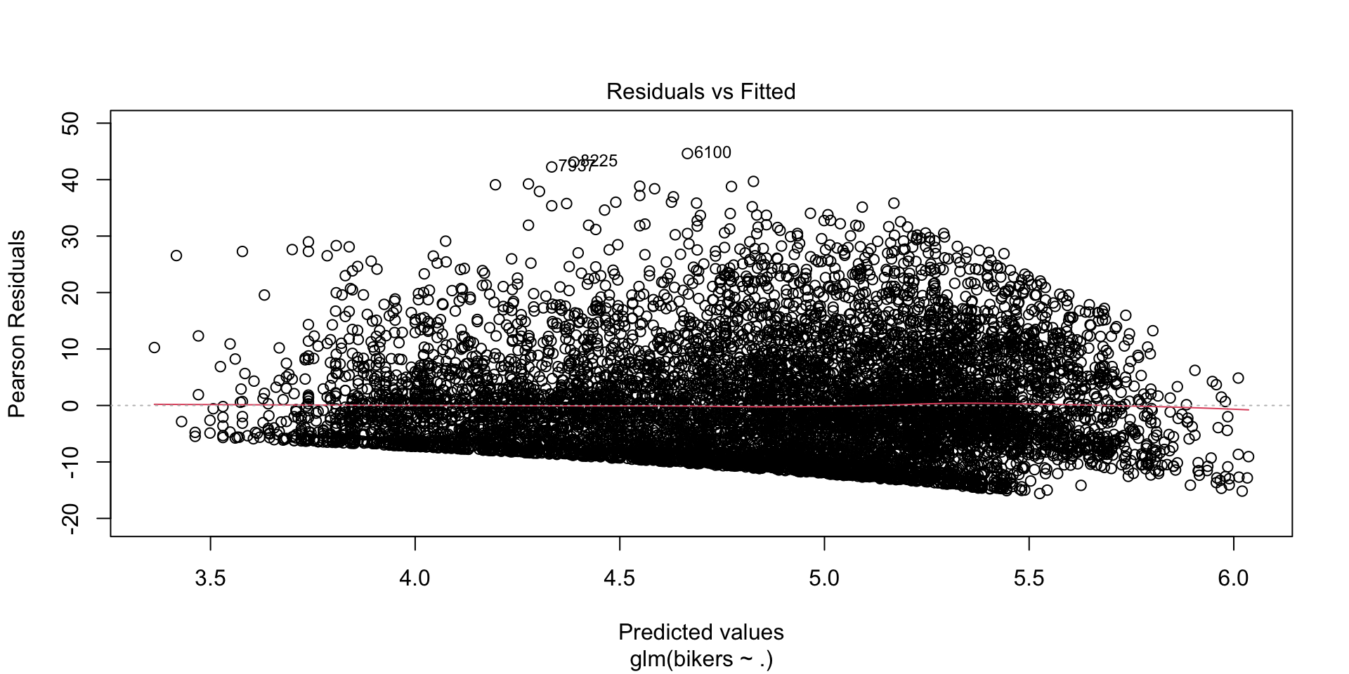
Residuals

The Poisson regression has the same problems as the Logistic Regression:

• responses are discrete (at least more than 2 values now)

• the variance is not constant

\[\text{resid}_{\text{raw}}= y_i - \hat{\lambda}_i, \quad\quad \text{resid}_{\text{pearson}}= \frac{y_i - \hat{\lambda}_i}{\sqrt{\hat{\lambda}_i}}\]

Residual plot

plot(bikers_poisson,1)

Overdispersion

The variance of a Poisson random variable equals the mean, which in practice may not be observed.

Poisson regression usually exhibits overdispersion.

An easy way to check is to fit a model using the quasilikelihood method and check if the dispersion parameter is very different from 1.

in R

bikers_quasipoisson <- glm(bikers ~ .,
                          data = bikeshare,
                          family = quasipoisson)

summary(bikers_quasipoisson)

Call:
glm(formula = bikers ~ ., family = quasipoisson, data = bikeshare)

Coefficients:
            Estimate Std. Error t value Pr(>|t|)    
(Intercept)  3.34536    0.03789  88.286  < 2e-16 ***
season2      0.06292    0.03561   1.767 0.077302 .  
season3     -0.14127    0.04112  -3.435 0.000595 ***
season4      0.37942    0.03196  11.872  < 2e-16 ***
workingday1 -0.03625    0.01848  -1.962 0.049849 *  
temp         2.68805    0.07077  37.981  < 2e-16 ***
windspeed    0.74145    0.07022  10.558  < 2e-16 ***
---
Signif. codes:  0 '***' 0.001 '**' 0.01 '*' 0.05 '.' 0.1 ' ' 1

(Dispersion parameter for quasipoisson family taken to be 90.60984)

    Null deviance: 1052921  on 8644  degrees of freedom
Residual deviance:  783300  on 8638  degrees of freedom
AIC: NA

Number of Fisher Scoring iterations: 5

Summary

Scroll down to see full content

• A count response can be modelled using a Poisson Regression

• The (conditional) expectation of a count response is the (conditional) mean counts.

• The (conditional) expectation of a count response equals the (conditional) variance

• A LR can not be used to model the conditional expectation of a count response since its range extends beyond positive values

• Instead, one can model a function of the conditional mean counts. A common choice in Poisson regression is to use the log function

Summary (cont.)

The interpretation of the coefficients depends on the type of variables and the form of the model:

The raw estimated coefficients (of the log-mean count model) are interpreted as:

• estimated log-mean counts of a reference group
• difference of estimated log-mean counts of a treatment vs a control group
• association between unit change in the input and changes in estimated log-mean counts

Summary (cont.)

The estiamted exponentiated coefficients (of the mean count model) are interpreted as:

• estimated averages counts of a reference group
• ratio of estimated averages counts of a treatment vs a control group
• multiplicative changes in estimated averages counts per unit change in the input

Summary (cont.)

• The estimated Poisson model can be used to make inference using the Wald’s satistic: confidence intervals and tests

• There are different type of fitted values (log-mean counts or counts?) and residuals

• Overdispersion is a potential problem in Poisson regression. Using quasilikelihood approach usual helps.