Prediction Uncertainty

Confidence Intervals for Prediction and Prediction Intervals

Last week

We learned 2 important topics

inference after model selection (double-dipping problem)
regularized methods

Last week in a nutshell

(you still need to know everythings covered in previous classes)

The post-inference problem

we run a simulation study and showed that the type I error rate got seriously inflated when the same data is used to select variables and conduct inference.

This problem is known as the post-inference problem (aka “doble dipping”)

the inference results computed on reused data are not valid (as seen in the first part of the worksheet).
A solution: if we split the data, we can use one part to select and the other part to estimate and build tests.
we showed with a simulation study that the type I error rate was controlled with this strategy.

Variable Selection Methods

Scroll down to see full content

Stepwise Selection Algorithms add (or remove) variables sequentially. They compare models of the same size using RSS and models of different sizes using appropriate metrics (e.g., adj$R^2$, AIC, BIC, $C_p$)
- different algorithms depending on the type of covariates (e.g., categorical with multiple levels)
Regularized Methods smoothly shrink the estimated coefficients. They minimize the RSS but subject to a bound on the size of the coefficients
- Ridge uses an $L_2-$norm to measure the size of the coefficients \[\lVert \beta \rVert_2^2 = \sum_{j = 1}^{p} \beta_j^2\]
- Lasso uses an $L_1-$norm to measure the size of the coefficients \[\lVert \beta \rVert_1 = \sum_{j = 1}^{p} |\beta_j|\]

Minimization subject to a bound on the size of the coefficients

Coefficients are shrunk as the level of penalty increases

iClicker

The value of the estimated coefficient at the dotted line correspond to the least squared estimated coefficients (OLS) calculated with lm() function

A. TRUE

–> B. FALSE

The bound (or equivalently, level of penalty $\lambda$) is usually selected by cross-validation aiming to minimize the MSE
With enough penalization, LASSO shrinks all estimated coefficients to zero. A way to select variables!
Ridge will never reach a value of zero and thus can not be used to select variables.
This “shrinkage” process biases the estimated coefficients to favor prediction performance.

Debiasing LASSO

Scroll down to see full content

iClicker: postLASSO estimator is a LS estimator on the selected variables, thus it’s unbiased

–> A: TRUE

B: FALSE

We can fit a LS estimator using only the variables selected by LASSO. This estimator is known as postLASSO and is unbiased!
If we want to make inference with postLASSO, we need to split the data!

Prediction Uncertainty

Today

Predictions using the estimated models depend on the sample used, thus it is subject to sample-to-sample variation

We’ll take into account the associated uncertainty using:

confidence intervals for prediction (CIP)
prediction intervals (PI)

What is the difference between these??

Predictions are random variables

We learned how to estimate a model using a random sample.

the estimated model can be used to predict the response of new observations.
the predictions depend on the random sample used! In other words, the predictions are functions of the a random sample.

Which means that the predictors are also random variables

Prediction uncertainty

A different sample would result in a different estimated model and, thus, different predictions!

the sample-to-sample variation in the estimated coefficients translates into variation in the predictions
we can account and report this uncertainty of the predictions using intervals

We’ll focused on predictions using MLR. Extensions to GLMs are not easy.

Dataset

In worksheet_09, you’ll work with the 2015 Property Tax Assessment from Strathcona County Dataset

The dataset contains data on property tax-assessed values in Strathcona County in 2014.


The Property Tax Assessment dataset has information about 27699 properties

                                       the_geom TAX_YEAR    ROLL_NUM
1 POINT (-113.27665515325147 53.54627975402534)     2015 -2147483648
         ADDRESS YEAR_BUILT  ASSESSCLAS           BLDG_DESC BLDG_METRE
1 447 CASCADE CR       2010 Residential 2 Storey & Basement        201
  BLDG_FEET GARAGE FIREPLACE BASEMENT BSMTDEVL ASSESSMENT LATITUDE LONGITUDE
1      2162      Y         Y        Y        N     580000 53.54616 -113.2769
  assess_val
1        580

To learn concepts from this topic, we’ll treat the entire dataset as a finite population and draw a random sample from it to estimate and predict population quantities.

set.seed(561) # DO NOT CHANGE THIS.

properties_sample <- 
    properties_data %>%
    slice_sample(n = 100, replace = FALSE)

We do NOT do this in practice. If we know the population we don’t need to take a sample!

Population vs Estimated SLR

You can estimate the population SLR using the sample properties_sample
You can compute the population coefficients of the SLR using all properties in properties_data

Again, in practice you would not be able to compute the population coefficients

lm_pop <- lm(assess_val ~ BLDG_METRE, properties_data)
lm_sample <- lm(assess_val ~ BLDG_METRE, properties_sample)

tidy(lm_pop) %>% 
    mutate_if(is.numeric, round, 3)

# A tibble: 2 × 5
  term        estimate std.error statistic p.value
  <chr>          <dbl>     <dbl>     <dbl>   <dbl>
1 (Intercept)    98.4      2.04       48.1       0
2 BLDG_METRE      2.56     0.012     207.        0

tidy(lm_sample) %>% 
    mutate_if(is.numeric, round, 3)

# A tibble: 2 × 5
  term        estimate std.error statistic p.value
  <chr>          <dbl>     <dbl>     <dbl>   <dbl>
1 (Intercept)    34.5     38.1       0.905   0.367
2 BLDG_METRE      3.07     0.228    13.4     0

Prediction of assessed value

Using linear regression, the assessed value of a random house in Strathcona can be modelled as the average assessed value of a house with similar characteristics plus some random error.

Mathematically,

\[Y_i = E[Y_i|X_{i}] + \varepsilon_i\]

The error, $\varepsilon_i$, is used to model fluctuations around the average population value of residencies of the same size.

If we assume that the conditional expectation is linear, then:

\[ E[Y_i|X_{i}] = \beta_0 + \beta_1 X_{i}\]

which is the population regression line!

Estimated SLR

We use the random sample to estimate the regression line.

The estimated SLR can be used to predict the value of any house in the county.

The prediction of the $i$-th property is given by:

\[\hat{Y}_i = \hat{\beta}_0 + \hat{\beta}_1 X_{i}\]

in practice, $\varepsilon_i$ will always be unknown since, $E(Y_i|X_i)$ is unknown
the residuals $r_i$ can be computed from the observed and predicted responses

Intervals to describe uncertainty

What do we want to predict with $\hat{Y}_i$? In general, we are interested in predicting either:

the average assessed value of a house of this size: $E[Y_i|X_i]$
the actual value of a house of this size: $Y_i$ (knowing its size $X_i$)

We predict both with uncertainty!

iClicker question

Which one do you think is more difficult to predict? Why?

A. It is more difficult to predict the average assessed value

—> B. It is more difficult to predict the actual assessed value

C. They are equally uncertain and difficult to predict

Confidence Intervals for Prediction

CIP are used when we want to predict $E[Y_i|X_i]$ (conditional expectation)!

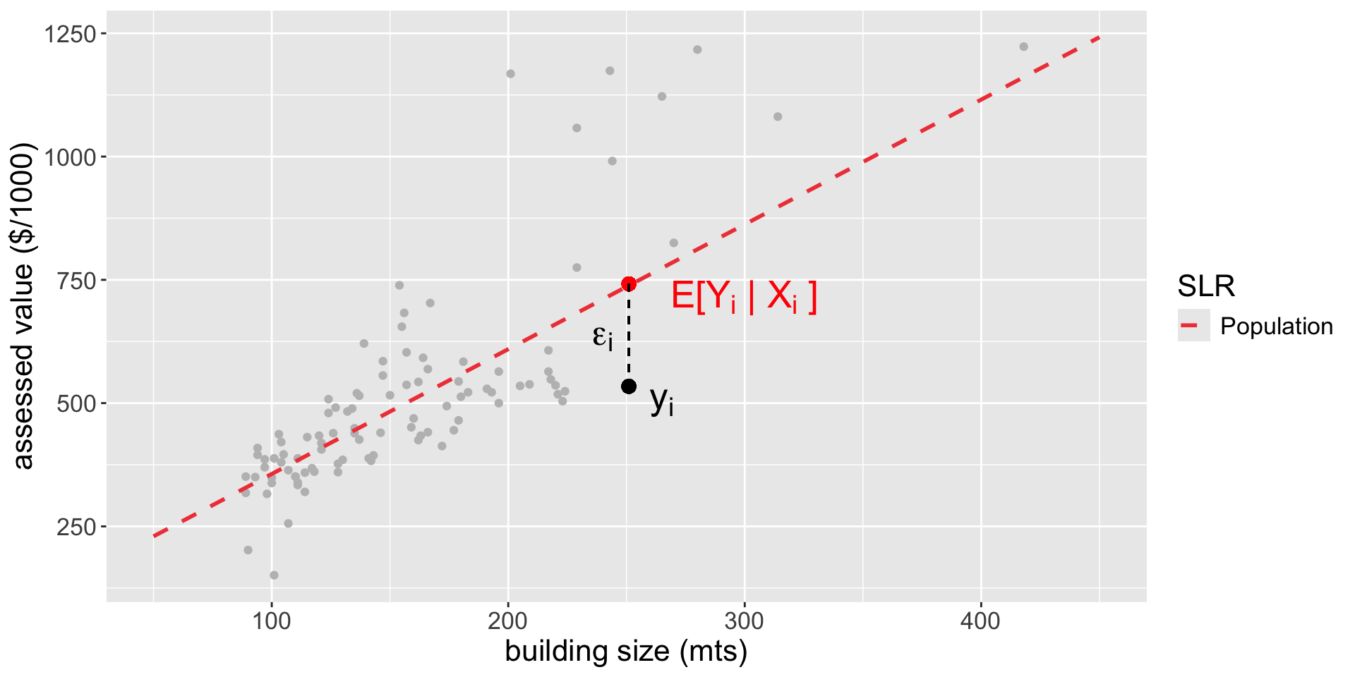
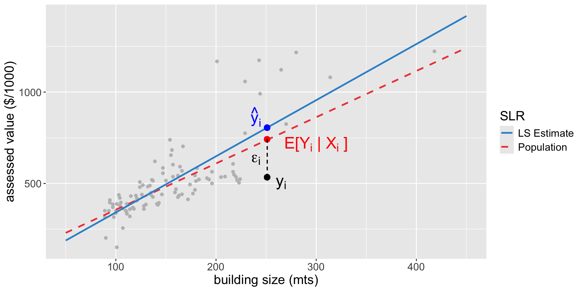
The predicted value $\hat{Y}_i = \hat{\beta}_0 + \hat{\beta}_1 X_{i}$ approximates, with uncertainty, the population average value $E[Y_i| X_{i}] = \beta_0 + \beta_1 X_{i}$

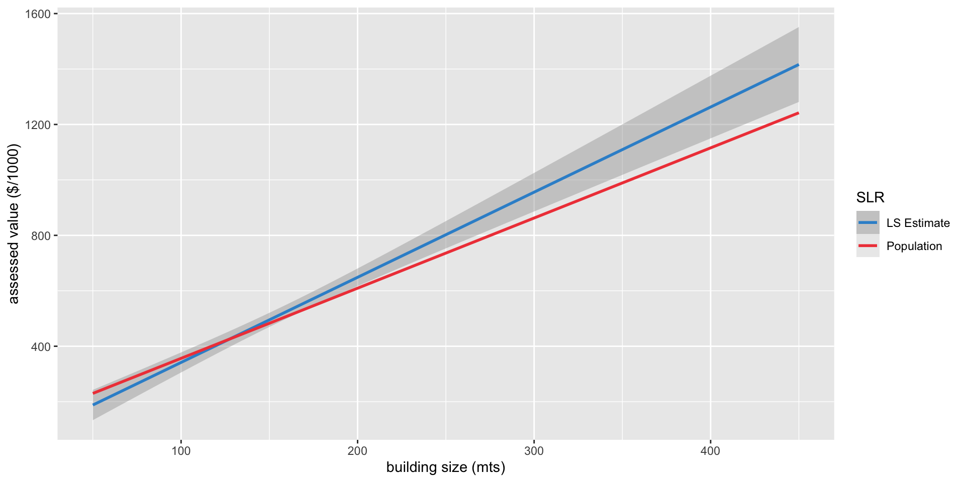
if we take a different sample, we get different estimates (i.e., different blue lines) and, consequently, different predictions

The only source of variation here is the sample-to-sample variation

A 95% confidence interval for prediction is a range that has a 95% probability of capturing the population average value of a house with size $X_i$

Once we have estimated and predicted values, the range is non-random so we use the word confidence (instead of “probability”) since nothing else is random!

Intervals for conditional expectations

properties_cip <- 
    properties_sample  %>% 
    select(assess_val, BLDG_METRE) %>% 
    cbind(predict(lm_sample, interval="confidence", se.fit=TRUE)$fit)

assess_val	BLDG_METRE	fit	lwr	upr
536	220	710.071	671.944	748.198
370	97	332.341	295.214	369.467
318	89	307.773	267.914	347.632

Interpretation for row 1:

With 95% confidence, the average value of a house of size 220 mts is between $\$671,944$ and $\$748,198$ (rounded)

Prediction Intervals

PI are used when we want to predict the actual response of a new observation $Y_i$!

The predicted value $\hat{Y}_i = \hat{\beta}_0 + \hat{\beta}_1 X_{i}$ also approximates, with uncertainty, the actual response $Y_i = \beta_0 + \beta_1 X_{i} + \varepsilon_i$.

However, now the uncertainty comes from the estimation (sample-to-sample variability) and the error term that generates the data, two sources of uncertainty!!

Two sources of uncertainty:

uncertainty 1: because the estimated value $\hat{\beta}_0 + \hat{\beta}_1 X_i$ approximates the average (population) value $\beta_0 + \beta_1 X_i$.
uncertainty 2: because the actual observation $Y_i$ differs from the population average value by an error $\varepsilon_i$

PIs are centered at the fitted value $\hat{Y}_i$ as well, but they are wider than the CIP to account for the extra source of uncertainty

A 95% prediction interval is a range within which a new value of a house of this size is expected to fall with a specified probability (e.g., 95%).

This time, the aim is to predict the actual response, which is a random variable, thus we interpret the interval in terms of “probability”.

properties_pi <- 
    properties_sample  %>% 
    select(assess_val, BLDG_METRE) %>% 
    cbind(predict(lm_sample, interval="prediction"))

assess_val	BLDG_METRE	fit	lwr	upr
536	220	710.071	454.519	965.622
370	97	332.341	76.937	587.745
318	89	307.773	51.957	563.588

Interpretation for row 1:

With 95% probability, the value of a house of size 220 mts is between $\$454,519$ and $\$965,622$ (rounded).

iClicker question

Which intervals are wider?

A. CIP are wider than PI since predicting an average value is less uncertain

B. CIP are wider than PI since predicting an average value is more uncertain

—> C. PI are wider than CIP since predicting an actual value is more uncertain

D. PI are wider than CIP since predicting an actual value is less uncertain

Conclusions

Confidence intervals for prediction account for the uncertainty given by the estimated LR to predict the conditional expectation of the response
Prediction intervals account for the uncertainty given by the estimated LR to predict the actual response, i.e, the conditional expectation of the response plus the error that generates the data!
PIs are wider than CIPs; both are centered at the fitted value!