Model Selection

Regularization Methods

Last week: stepwise selection

We learned how to select a model using stepwise algorithms

these are greedy algorithms
results depend on the order in which variables are selected
variables are either in or out

If we can think out as the estimated coefficient being \(0\), can we smoothly shrink the estimator instead of selecting between a value and \(0\)?

Today: regularization methods

Regularized methods
Can we select and train models at once?
Biased estimators

Dataset

Let’s use part of the Ames Housing dataset to introduce and illustrate regularized methods.

# A tibble: 6 × 6
  LotFrontage LotArea MasVnrArea TotalBsmtSF GrLivArea SalePrice
        <dbl>   <dbl>      <dbl>       <dbl>     <dbl>     <dbl>
1          50    8500          0         649      1317     40000
2          65    6040          0           0      1152     82000
3          33    4456          0         736      1452    113000
4          52    6240          0         816      1176    114500
5         110    8472          0         816       816    110000
6          60    7200          0         780       780    124900

Stepwise Selection

Let’s use the “forward” selection algorithm on this (smaller) training set to select some of the variables to predict SalePrice

Housing_forward_sel <- regsubsets(
  x = SalePrice ~ ., nvmax = 19,
  data = training_Housing[,c(1:5,20)],
  method = "forward",
)

summary(Housing_forward_sel)[[1]]

  (Intercept) LotFrontage LotArea MasVnrArea TotalBsmtSF GrLivArea
1        TRUE       FALSE   FALSE      FALSE       FALSE      TRUE
2        TRUE       FALSE   FALSE      FALSE        TRUE      TRUE
3        TRUE       FALSE   FALSE       TRUE        TRUE      TRUE
4        TRUE       FALSE    TRUE       TRUE        TRUE      TRUE
5        TRUE        TRUE    TRUE       TRUE        TRUE      TRUE

Coefficients of selected variables

coef(Housing_forward_sel,1)

(Intercept)   GrLivArea 
   816.3893    119.0938

coef(Housing_forward_sel,2)

 (Intercept)  TotalBsmtSF    GrLivArea 
-40522.44180     83.88263     88.12881

The estimated coefficient for TotalBsmtSF “jumps” from 0 to 83.88.

Similarly for other coefficients in other steps.

Can the selection be done more “smoothly”??

Regularization methods!!

Regularization (or penalized or shrinkage) shrink coefficients in a continuous way by adding a penalty to the objective funcion.

Mathematically, instead of minimizing the RSS

\[ \ \min_{\beta_0, \boldsymbol{\beta}} \ \sum_{i=1}^n \left(Y_i - \beta_0 - \boldsymbol{X}_i \boldsymbol{\beta} \right)^2 \]

we minimize the penalized RSS, for example:

\[ \sum_{i=1}^n \left(Y_i - \beta_0 - \boldsymbol{X}_i \boldsymbol{\beta} \right)^2 + \ \overbrace{\lambda \ \sum_{j=1}^p \, \beta_j^2}^{penalty} \ \]

Ridge vs LASSO: penalty

We’ll focus on 2 methods (there are many other penalty functions one can use!)

Ridge uses an \(L_2-\)norm to measure the size of the coefficients \[\lVert \beta \rVert_2^2 = \sum_{j = 1}^{p} \beta_j^2\]
Lasso uses an \(L_1-\)norm to measure the size of the coefficients \[\lVert \beta \rVert_1 = \sum_{j = 1}^{p} |\beta_j|\]

Ridge vs LASSO: objective function

Ridge

\[ \sum_{i=1}^n \left(Y_i - \beta_0 - \boldsymbol{X}_i \boldsymbol{\beta} \right)^2 + \ \overbrace{\lambda \ \sum_{j=1}^p \, \beta_j^2}^{penalty} \ \]

LASSO

\[ \sum_{i=1}^n \left(Y_i - \beta_0 - \boldsymbol{X}_i \boldsymbol{\beta} \right)^2 + \ \overbrace{\lambda \ \sum_{j=1}^p \, |\beta_j|}^{penalty} \ \]

The penalty parameter

Scroll down to see full content

How much to shrink??

\(\lambda\) is called the penalty parameter
If \(\lambda = 0\), the objective function of the shrinkage methods is the same as that of LS!! Same estimators!!
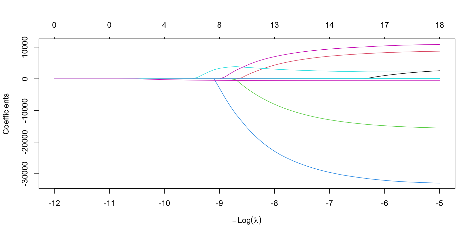
As \(\lambda\) grows, coefficients are shrunk.
- LASSO eventually shrinks them all to zero
- Ridge will never reach a value of zero
The penalty parameter \(\lambda\) can be selected using the data. This process is called “tuning”.
- an option is to select the value that yields the smallest \(\text{MSE}_{\text{test}}\).
- this tuning is done using an internal cross-validation or a validation set so that the model does not use test data

Equivalently, we can think that we impose a bound on the size of the coefficients.

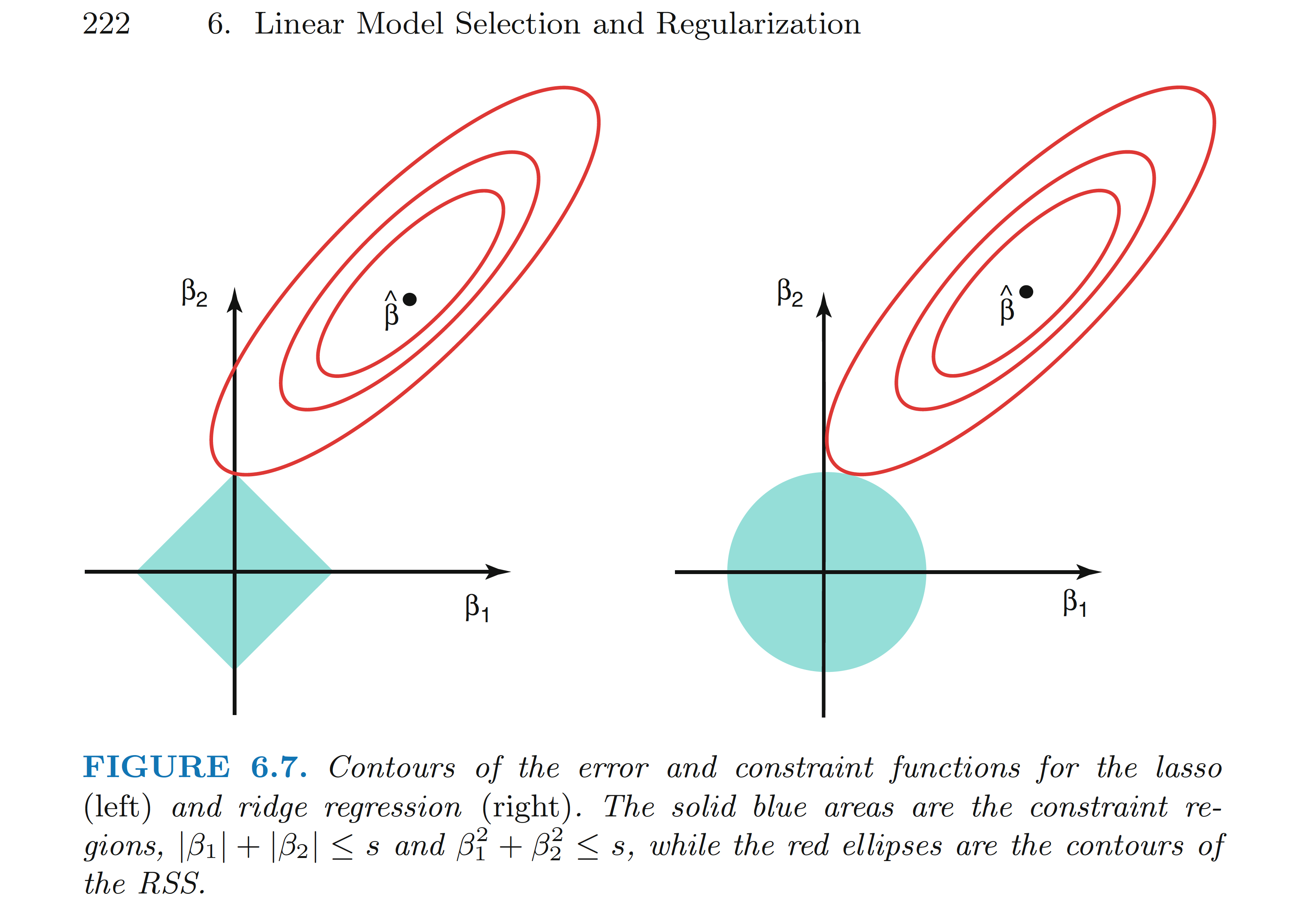
Figure from ISLR book

Ridge

Proposed in 1970 by Hoerl, A.E. and Kennard, R. in
It does not shrink parameters to \(0\), so it does not select variables
It has been proposed as a method to address multicollinearity problems (we’ll skip the math)

LASSO

The least absolute shrinkage and selection operator

Proposed in 1996 by Tibshirani in
it does shrink coefficients to \(0\), thus it can be used to simultaneously select and train (estimate) a model!!
It has been proposed as a method to select strong predictive models

Bias

This “shrinkage” process biases the estimated coefficients!

we sacrifice bias for a lower variance to potentially gain prediction performance!!

Important: since the method depend on the size of the coefficients, we need to standardize the input variables (default option)

In R

Scroll down to see full content

To build a regularized regression we can use the package glmnet in R. Check this useful vignette

the glmnet() function requires: a matrix with input variables and a vector of responses
the argument alpha = 1 corresponds to a LASSO penalty and alpha = 0 for a Ridge penalty

There are infinite other options in between known as Elastic Net

glmnet() selects a grid of \(\lambda\) values by default or you can specify one
it is recommended to use given extraction fuctions to obtain the objects, e.g., estimated coefficients
the function cv.glmnet() can be used to find an “optimal” value of \(\lambda\) by cross-validation

CV creates many test sets from the training set (we’ll see CV later)

we can visualize how the estimated test MSE changes for different values of \(\lambda\)

Step 1 -3

create matrices
set alpha = 1 for LASSO
create a grid of lambda values (try using the default as well)

Housing_X_train <- as.matrix(training_Housing[,-20])
Housing_Y_train <- as.matrix(training_Housing[,20])

Housing_X_test <- as.matrix(testing_Housing[,-20])
Housing_Y_test <- as.matrix(testing_Housing[,20])

Housing_LASSO <- glmnet(
  x = Housing_X_train, y = Housing_Y_train,
  alpha = 1,
  lambda = exp(seq(5, 12, 0.1))
)

plot(Housing_LASSO)

Step 4

Scroll down to see full content

extract estimated coefficients for a given level of regularization

20 x 1 sparse Matrix of class "dgCMatrix"
                   s=40000
(Intercept)   1.116881e+05
LotFrontage   .           
LotArea       .           
MasVnrArea    .           
TotalBsmtSF   1.447926e+01
GrLivArea     3.126415e+01
BsmtFullBath  .           
BsmtHalfBath  .           
FullBath      .           
HalfBath      .           
BedroomAbvGr  .           
KitchenAbvGr  .           
Fireplaces    .           
GarageArea    9.785771e+00
WoodDeckSF    .           
OpenPorchSF   .           
EnclosedPorch .           
ScreenPorch   .           
PoolArea      .           
ageSold       .

Step 5

select the best lambda by CV

Housing_cv_LASSO <- cv.glmnet(
  x = Housing_X_train, y = Housing_Y_train,
  alpha = 1,
  lambda = exp(seq(5, 12, 0.1))
)

plot(Housing_cv_LASSO, main = "Lambda selection by CV with LASSO\n\n")

Minimizing the MSE

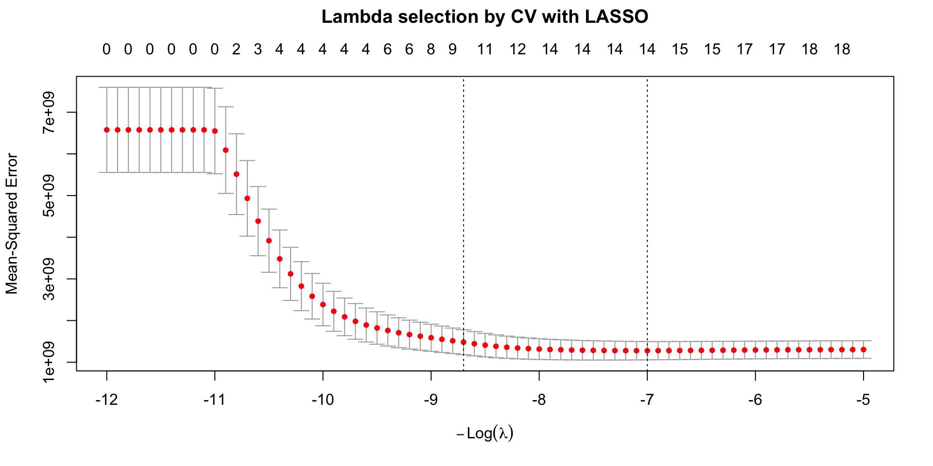
The plot shows the estimated (by CV) test mean squared error (MSE, \(y\)-axis) for a grid of values of \(\lambda\) (\(x\)-axis on the natural log-scale).

the numbers at the top \(x\)-axis indicate the number of inputs whose estimated coefficients are different from zero for different values of \(\lambda\).

the error bars represent the variation across the different test sets of the CV (folds)

Selection of penalty level

The two vertical dotted lines correspond to two values of \(\lambda\):

\(\hat{\lambda}_{\text{min}}\) which provides the minimum MSE in the grid.
\(\hat{\lambda}_{\text{1SE}}\) largest value of lambda such that the corresponding MSE is within 1 standard error of that of the minimum (more penalization at a low cost)

round(Housing_cv_LASSO$lambda.min, 2)

[1] 1096.63

round(log(Housing_cv_LASSO$lambda.min),2)

[1] 7

LASSO “smoothly” selects variables and trains the corresponding model for the values of lambda in the grid

plot(Housing_cv_LASSO$glmnet.fit, "lambda")
abline(v = log(Housing_cv_LASSO$lambda.min), col = "red", lwd = 3, lty = 2)

Step 5 targeted

5’. extract the estimated coefficients that minimize the CV-test MSE (or the 1SE option).

coef(Housing_cv_LASSO, s = "lambda.min")

20 x 1 sparse Matrix of class "dgCMatrix"
                lambda.min
(Intercept)    44109.52081
LotFrontage        .      
LotArea            1.74035
MasVnrArea        32.59693
TotalBsmtSF       37.95458
GrLivArea         80.90134
BsmtFullBath    9407.91300
BsmtHalfBath       .      
FullBath        7159.11808
HalfBath           .      
BedroomAbvGr  -12964.72474
KitchenAbvGr  -29590.90301
Fireplaces      2414.90241
GarageArea        46.58762
WoodDeckSF        10.59831
OpenPorchSF       20.08263
EnclosedPorch      .      
ScreenPorch        .      
PoolArea          73.23908
ageSold         -489.95991

Prediction

LASSO was proposed as a method to build strong predictive models. Let’s use it to predict SalePrice in the test set.

Housing_test_pred_LASSO_min <- 
            predict(Housing_cv_LASSO, 
            newx = Housing_X_test, 
            s = "lambda.min")
tibble(Housing_Y_test,LASSO_prediction = Housing_test_pred_LASSO_min) %>% head()

# A tibble: 6 × 2
  Housing_Y_test[,"SalePrice"] LASSO_prediction[,"lambda.min"]
                         <dbl>                           <dbl>
1                       223500                         231772.
2                       140000                         164854.
3                       129900                         153479.
4                       118000                          93876.
5                       279500                         239443.
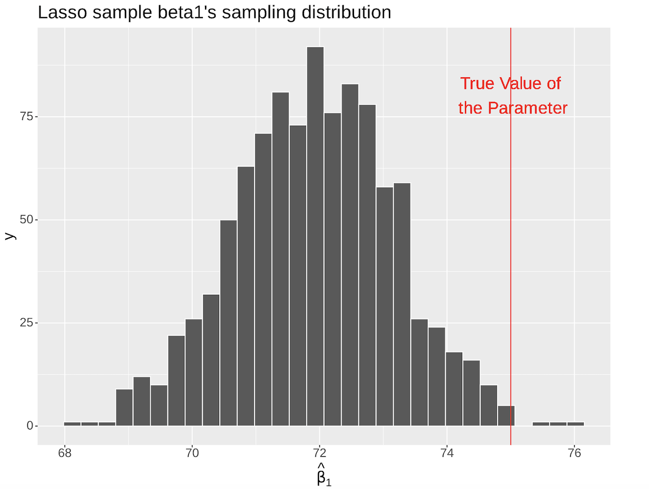
6                       132000                          98443.

Can we use LASSO for inference??

The main drawback of using LASSO for inference is that the estimated coefficients are biased. (in worksheet_08)

The `map` function

In the worksheet and tutorial, you’ll simulate data to explore different problems related to model selection.

the function map applies different funtions to a list of datasets (identified by the replicate variable)
the output of map is also a list

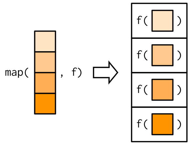
Image from Advaced R, by H. Wickham

For example (from your worksheet)

full_models <- 
    dataset %>% 
    group_by(replicate) %>% 
    nest() %>% 
    mutate(models = map(.x = data, ~ lm(Y ~ ., data = .x)))`

map is used to fit LS to each dataset using the function lm (f in the figure)
the output is a list containing the elements replicate, data, and models (the fitted models)!!

Model Selection

Last week: stepwise selection

Today: regularization methods

Dataset

Stepwise Selection

Coefficients of selected variables

Regularization methods!!

Ridge vs LASSO: penalty

Ridge vs LASSO: objective function

The penalty parameter

Ridge

LASSO

Bias

In R

Step 1 -3

Step 4

Step 5

Minimizing the MSE

Selection of penalty level

Step 5 targeted

Prediction

Can we use LASSO for inference??

The map function

For example (from your worksheet)

The `map` function