Logistic regression is a powerful statistical method used for modelling a binary (and binomial) response variable.
For example, we can use a logistic regression to
compare the presence of bacteria between groups taking a new drug and a placebo, respectively.
Response: present or not present
predict whether or not a customer will default on a loan given their income and demographic variables.
Response: default or not default
know how GPA, ACT score, and number of AP classes taken are associated with the probability of getting accepted into a particular university.
Response: accepted or not accepted
The response
Scroll down to see full content
To fit a logistic regression in R, the response needs to be a numerical variable (0 and 1) or a factor, with two levels (since R stores factors as integers).
For example, a numerical binary response \(Y_i\) that flags the successes (S) has the form:
model_titanic_logistic <-glm(formula = survived ~ fare, data = titan, family ='binomial')summary(model_titanic_logistic)
Call:
glm(formula = survived ~ fare, family = "binomial", data = titan)

Coefficients:
             Estimate Std. Error z value Pr(>|z|)
(Intercept) -0.941330   0.095129  -9.895  < 2e-16 ***
fare         0.015197   0.002232   6.810 9.79e-12 ***
---
Signif. codes:  0 '***' 0.001 '**' 0.01 '*' 0.05 '.' 0.1 ' ' 1

(Dispersion parameter for binomial family taken to be 1)

    Null deviance: 1186.7  on 890  degrees of freedom
Residual deviance: 1117.6  on 889  degrees of freedom
AIC: 1121.6

Number of Fisher Scoring iterations: 4
Interpretation: log-odds
The coefficients can be interpreted in terms of the log-odds (logit link):
Intercept\(\hat{\beta}_0 = -0.9413\): the estimated log-odds of surviving with a paid fare of 0 dollars is -0.9413.
Slope\(\hat{\beta}_1 = 0.0152\): an increase of 1 dollar in the fare paid is associated with an estimated increase in the log-odds of surviving of 0.0152.
same as for MLR but with response “log-odds of success”!
Important
Note the word “estimated” in the interpretation.
Interpretation: odds
A more natural way of interpreting the coefficients of a logistic regression is based on odds of success
Using basic algebra, the model can also be written as:
We need to exponentiate the coefficients to interprete them as changes in the odds. Find more details in the math appendix
Exponentating the coefficients
#Coefficients for the oddstidy(model_titanic_logistic, exponentiate =TRUE) %>%mutate_if(is.numeric, round, 3) %>% knitr::kable()
term
estimate
std.error
statistic
p.value
(Intercept)
0.390
0.095
-9.895
0
fare
1.015
0.002
6.810
0
Slope: \(e^{\hat{\beta}_1} = e^{0.0152} = 1.015\): we estimate that an increase of 1 dollar in the fare paid is associated with an increase of the odds of surviving by a factor of 1.015 (or with an increase of the odds of surviving of 1.5% percent )
Reference level: female, note the dummy variable name sexmale
Interpretation (in terms of odds)
Scroll down to see full content
Intercept: \(e^{\hat{\beta}_0} = e^{1.057} = 2.8765\), a female passenger had a an estimated odds of surviving equal to 2.8765 (i.e., estimated by proportion of female survivors relative to the proportion of female deaths in the sample)
Slope: \(e^{\hat{\beta}_1} = e^{-2.514} = 0.08097\), the estimated odds of surviving for a male passenger are 0.08097 times the estimated odds for a female passenger, corresponding to a decrease of \(91.90\%\) (note \((0.08097-1) \times 100 = - 91.90\)).
Or, The estimated odds of surviving for a female passenger are multiplied by a factor of 0.08097 for a male passenger.
Odds ratio: note that \(e^{\hat{\beta}_1} = 0.08097 = \frac{\text{odds}_\text{male}}{\text{odds}_\text{female}}\)
turning to odds of failure: for a male passanger the estimated odds of dying are \(e^{2.514} = 12.3542\)times higher than of those of females
More details about these equivalences are given in the math appendix
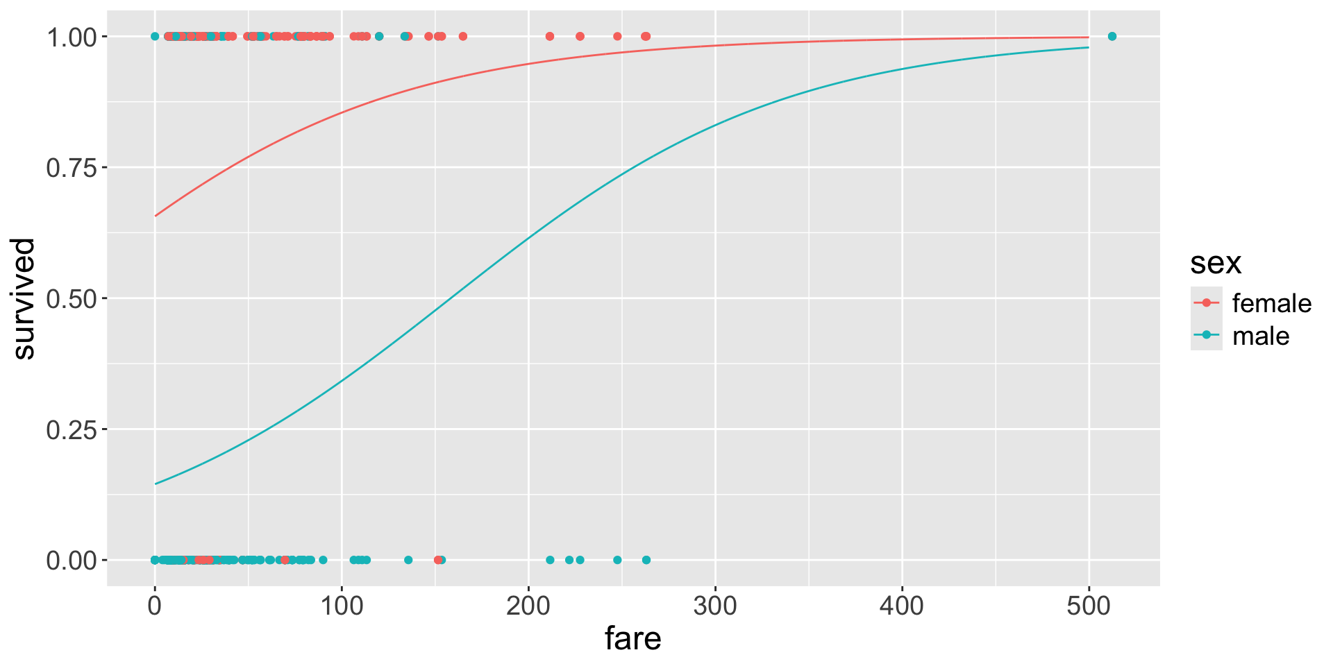
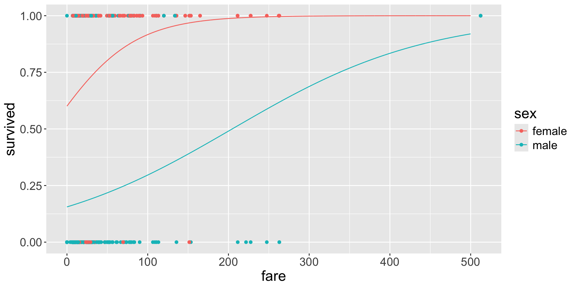
Case 3: one categorical and one numerical covariate
Let’s fit a logistic regression using sex and fare (omiting subscript \(i\) for simplicity)
for male passengers, increasing the fare in 1 dollar is associated with an estimated increase of the odds of surviving by a factor of\(e^{0.008} = 1.008\).
for male passengers, increasing the fare in 1 dollar is associated with an estimated increase in the odds of surviving of \(0.8\%\).
Using exponentiated coefficients
Note that you can also recover both curves using the exponentiated coefficients, from the tidy table, with exponentiate = TRUE.
For fare: \(p < 0.001\) indicating significant evidence to reject the null hypothesis that states that there is no association between fare and the log-odds of surviving, for either female or male passengers.
Inference for odds of success
Scroll down to see full content
You can also get confidence intervals for the exponenciated coefficients
We can be \(90\%\) confident that an increase of 1 dollar in fare is associated with a \(0.8\%\) to \(1.5\%\) increase in the odds of surviving for either male or female passengers.
since \((1.008-1)\times 100\%= 0.8\%\) and \((1.015-1)\times 100\%= 1.5\%\)
Summary
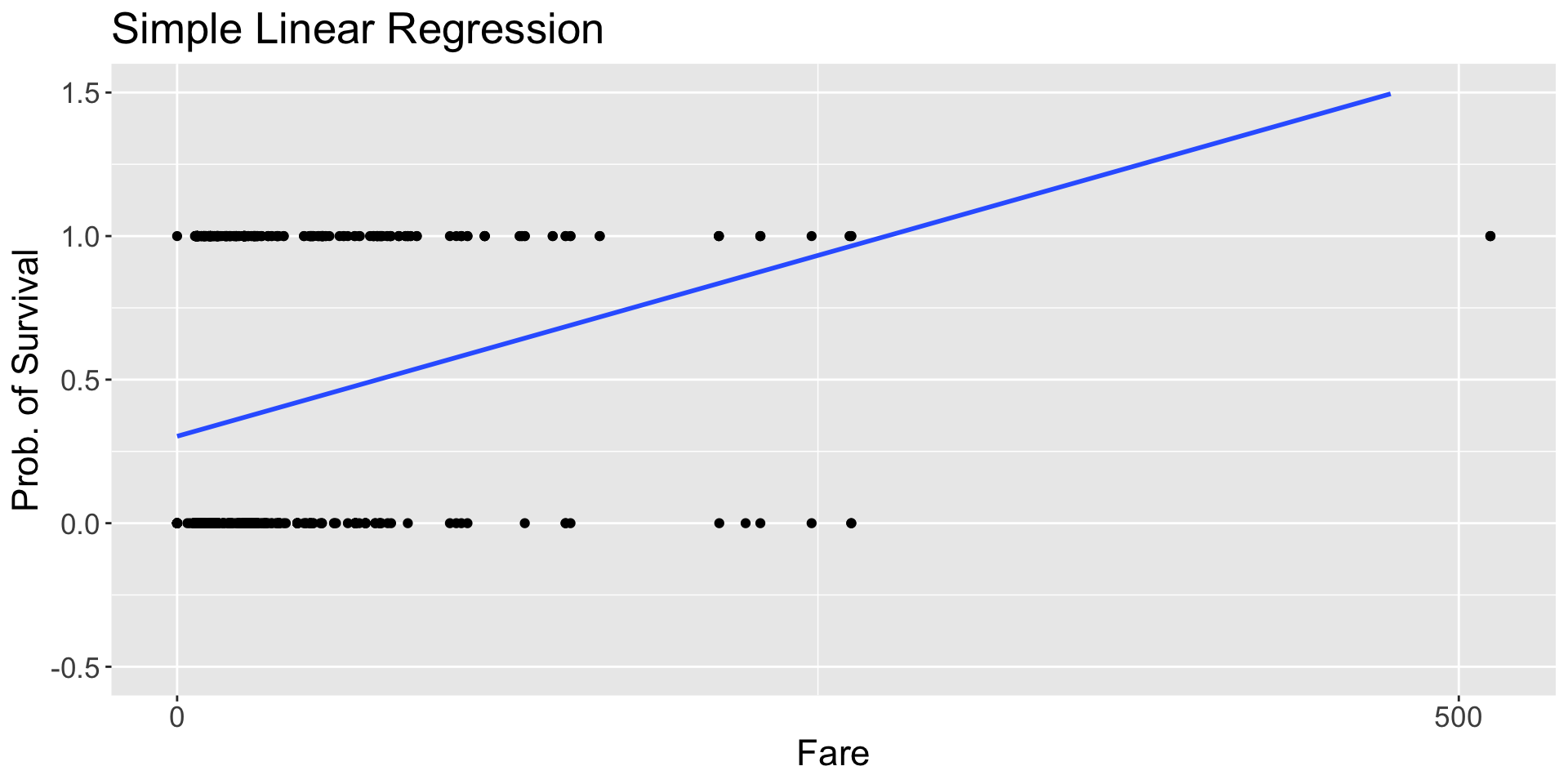
The (conditional) expectation of a binary response is the (conditional) probability of success.
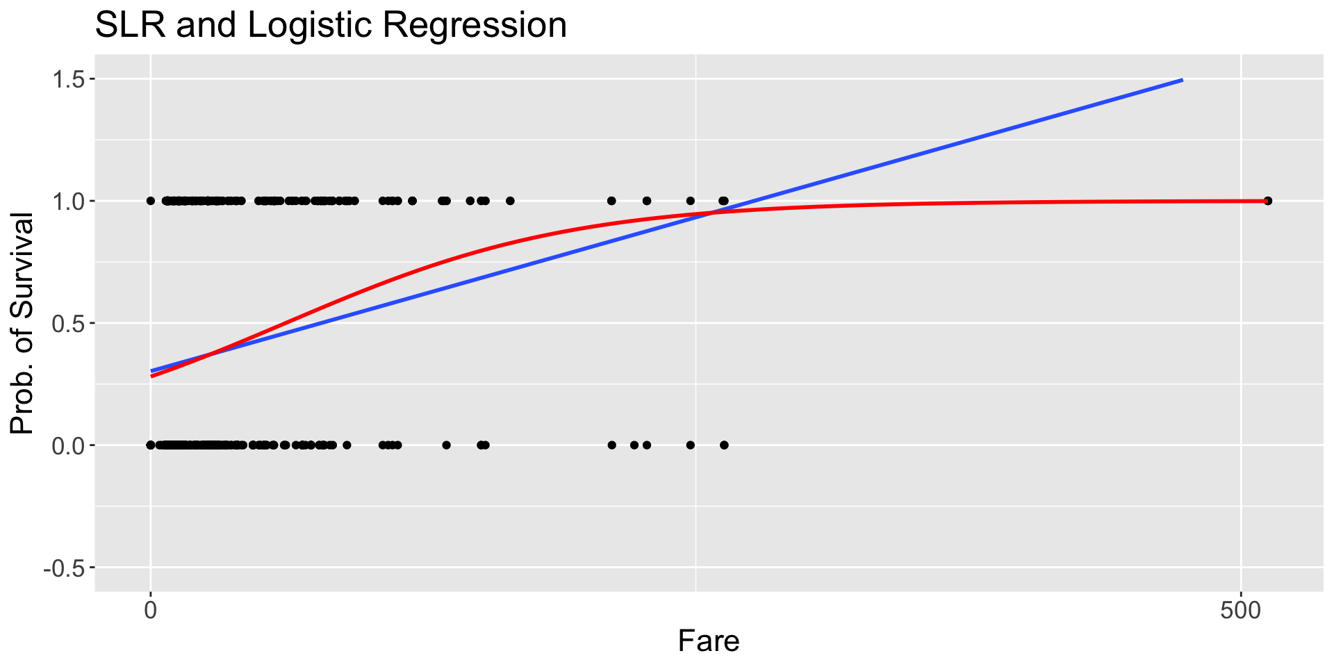
A MLR can not be used to model the conditional expectation of a binary response since its range extends beyond the interval \((0,1)\)
Instead, one can model a function of the conditional probability. A common choice in logistic regression is to use the logit function (logarithm of odds)
Summary (cont.)
Scroll down to see full content
The interpretation of the coefficients depends on the type of variables and the form of the model:
The raw coefficients (of the log-odds model) are interpreted as:
log-odds of a reference group
difference of log-odds of a treatment vs a control group
changes in log-odds per unit change in the input
The exponentiated coefficients (of the odds model) are interpreted as:
odds of a reference group
odds ratio of a treatment vs a control group
multiplicative changes in odds per unit change in the input
Important
Once you have an estimated model, remember to interprete results as “estimated” values.
Summary (cont.)
The estimated logistic model can be used to make inference about the population coefficients using the Wald’s satistic: confidence intervals and tests