STAT 301

Course Review

Statistical Modelling

3 models under a common framework

Model	Response	Distribution	Parameter	Linear
MLR	continuous	Normal	mean of response	identity
Logistic	binary	Bernoulli	probability of S	log-odds
Poisson	counts	Poisson	mean count	log

mean(house price) = $\beta_0$ + $\beta_1$size + $\beta_2$basementY
log(odds of default) = $\beta_0$ + $\beta_1$balance + $\beta_2$income + $\beta_3$studentY
log(mean(number of bikes)) = $\beta_0$ + $\beta_1$temperature

These functions are used to interpret the regression coefficients!!!

Interpretation

Model	continuous covariate
MLR	an increase of 1 unit in the covariate is associated with an estimated increase/decrease of $\|\hat{\beta}_1\|$ in the average response
Logistic	an increase of 1 unit in the covariate is associated with an estimated increase/decrease in the log odds of success by $\|\hat{\beta}_1\|$, or a change in the odds of success by a factor of $e^{\hat{\beta}_1}$
Poisson	an increase of 1 unit in the covariate is associated with an estimated increase/decrease in the log average counts by $\|\hat{\beta}_1\|$, or or a change in the mean counts by a factor of $e^{\hat{\beta}_1}$

Interpretation: examples

Scroll down to see full content

Logistic: a dollar increase in balance is associated with
- an increase in the estimated log odds of default by 0.0055, or
- an increase in the estimated odds of default by a factor of 1.0055,
- or an increase in the estimated odds of 0.55%
Poisson: a Celsius degree increase in temperature is associated with
- an increase in the estimated log mean number of bikes rented of 0.62, or
- an increase in the estimated mean number of bikes by a factor of 1.86 ($e^{0.62}$),
- or an increase in the estimated mean number of bikes of 86% ((1.86-1) $\times$ 100)

Key words

Scroll down to see full content

estimate or estimated (these are not population quantities, they depend on the sample)
associated with (if the data comes from an observational study causation can not be established)
“by a factor of” or “times” or “percent” if estimated coefficients are exponentiated
“holding other variables constant at any value” if the model is additive and has more variables, otherwise don’t!
check units!!

Additive models vs interactions

for additive models: coefficients are interpreted holding other variables constant at any value
for models with interactions: interpretations depend on levels or values of other variables, not at any value, not regardless of other variables!

Warning

Interaction terms do not model correlations between covariates!!

We use interactions when the association between a covariate and the response depends on another covariate(s)

Example of additive MLR

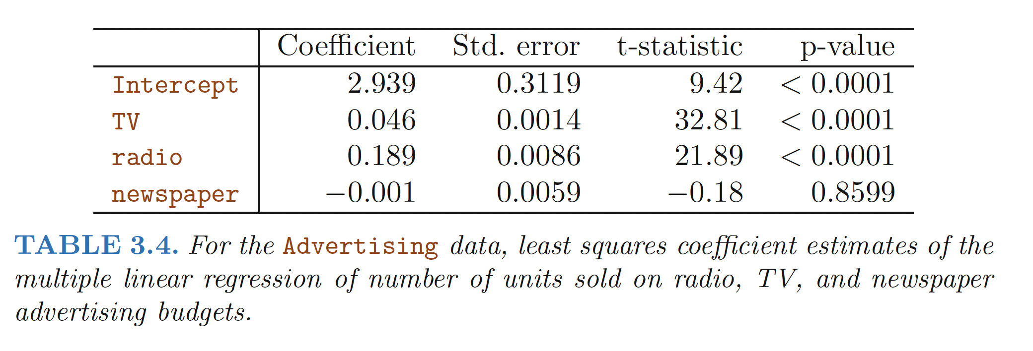
for any given amount of spending in TV and newspaper advertising, spending an additional $1000 on radio advertising is associated with an estimated increase in sales by approximately $189

or “keeping the spending in TV and newspaper advertising constant at any value”

Table from ISLR

Example of model with interaction

To be completed

Hypothesis tests and CI

We need the sampling distribution (distribution of the estimators of the regression coefficients, $\hat{\beta}_j$)

For the 3 models, we usually use a Normal approximation of the sampling distribution (details beyond this course)

for MLR: we usually need to estimate the variance of the error term ($\sigma$) and the sampling distribution becomes a $t$-student distribution
- we estimate $\sigma$ using the RMSE, given by glance()
for Logistic and Poisson: the variance of the response depends on their mean so we don’t need to estimate it separately. Given the CLT, we use a Normal approximation as the sampling distribution
- recall that sometimes we observe overdispersion (or underdispersion)

Interpretations of tests

Scroll down to see full content

The null hypothesis: $H_0: \beta_j = 0$

check the significance level
check the alternative hypothesis
the interpretion depends on the meaning of the coefficient
interpretations are for true coefficients, not estimates

We have statistically significant evidence (p-value < .001) that the mean number of fires is positively associated with temperature.

Remember that we never know what the true population parameters are! At a significance level:
- we have evidence to reject $H_0$. It doesn’t mean $H_1$ is true!
or
- we don’t have enough evidence to reject (we fail to reject) $H_0$. It doesn’t mean $H_0$ is true!

CIs of coefficients

Recall that once the data is collected, the intervals are not random and we interpret them in terms of confidence, not probabilities!

We are 95% confident that each additional degree in temperature is associated with an increase in the mean number of fires between 5% and 10%.

We can also use bootstrapping to compute CIs

Assumptions and Diagnosis

In worksheet_03 and tutorial_03 we used simulations to study:

Normality: only for MLR, not needed for estimation or large sample apprximations but the linear model will be a good fit if the assumption holds.
Homoscedasticity: only for MLR, the spread (or variance) of the errors in a model is the same across all levels of the covariate(s).
Confounding Factor: a variable related with a covariate and the response, and it can make it look like there’s an association between them, even if there isn’t.
Multicollinearity: correlation between covariates.
Independence: we assume that observations are independent of each other

Predictions and Residuals

Scroll down to see full content

Predictions are values of the response computed with the estimated model for fixed values of the covariates:
- fitted: common name for in-sample predictions
Residuals is the difference between the observed response and the fitted values
Fitted values and residuals can be computed for the 3 models: MLR, Logistic and Poisson
However: recall that different quantities can be predicted with logistic (log-odds, odds, probabilities) and Poisson (log-counts, counts). Check code for different versions!
In Logistic and Poisson, the variance of each observation depends on the covariates (not constant), so residuals are adjusted (e.g., Pearson, deviance). Check code for different versions!
See tutorial_04 and tutorial_05

After the midterm

Goodness of Fit: MLR

Many evaluation metrics used to evaluate MLR measure how far $y$ is from $\hat{y}$:

Residuals Sum of Squares: RSS = $\sum_{i=1}^n(y_i - \hat{y}_i)^2$
Residuals Standard Error: RSE = $\sqrt{\frac{1}{n-p-1} \text{RSS}}$
Mean Squared Error: MSE = $\frac{1}{n}\sum_{i=1}^n(y_i - \hat{y}_i)^2$
Coefficient of Determination, $R^2 = 1 - \frac{RSS}{TSS}$
Adjusted $R^2$: $\text{adj}R^2 = 1 - \frac{RSS/(n-p-1)}{TSS/(n-1)}$

For more details see Model Evaluation

Goodness of Fit: Logistic and Poisson

For Logistic and Poisson regression, we measure the distance between $y$ and $\hat{y}$ using the deviance.

The deviance generalizes the Residual Sum of Squares (RSS) defined for MLR.

Image from Notes for Predictive Modeling

For more details see Model Evaluation: Goodness of Fit for Logistic and Poisson

Selection: Nested Models

We can compare nested models testing the (simultaneous) significance of additional coefficients in the larger model

reduced: price ~ size

full: price ~ size + distance + years_since_built

Note

The full model contains all the variables in the reduced one plus some new variables (in bold fonts)
The null hypothesis states that the coefficients of both variables, distance and years_since_built, are equal to zero

Suppose that the reduced model has $q$ covariates and the full model has the same $q$ plus $s$ additional ones.

Is the full model significantly different from the reduced one??

\[H_0: \beta_{q+1} = \beta_{q+2} = \ldots = \beta_{q+s} =0\] For MLR: we can use an $F$-test to test this hypothesis (review worksheet_06 and tutorial_06)

For Logistic and Poisson: we use can use an $\chi^2$-test to test this hypothesis (review worksheet_07)

Note

In all cases you use anova(reduced, full) in R to compute the test
For Logistic and Poisson, you need to specify test = "Chisq"
Recall special cases: $F$-test vs $t$-test, reduced = intercept-only

Variable Selection Methods

Stepwise Selection Algorithms

Forward: starts with the intercept-only model and adds one variable at a time.
- It will stop when the number of selected covariates equals the number of observations
Backwards: starts with the full model and removes variables, one at a time.
- It can only be used if the number of observations is larger than the number of covariates.

For MLR: the RSS is used to add/remove variables (i.e., to compare models of the same size) and different measures can be used to compare models of different sizes (e.g., adj$R^2$, AIC, BIC, $C_p$)
For Logistic and Poisson: the AIC or BIC can be used to compare models

Note

We distinguished between the selection of generative models and predictive models, using different evalution metrics.
Review worksheet_07 for generative MLR models and tutorial_07 for generative MLR models
regsubsets() function from the leaps package in R can only be used for linear regression
stepAIC function from the MASS package in R can be used for the 3 models but is based on AIC and BIC only

Regularized Methods

Smoothly shrink the estimated coefficients. They minimize the RSS but subject to a bound on the size of the coefficients.

Ridge uses an $L_2-$norm to measure the size of the coefficients \[\lVert \beta \rVert_2^2 = \sum_{j = 1}^{p} \beta_j^2\]
Lasso uses an $L_1-$norm to measure the size of the coefficients \[\lVert \beta \rVert_1 = \sum_{j = 1}^{p} |\beta_j|\]

The bound (or equivalently, level of penalty $\lambda$) is usually selected by cross-validation aiming to minimize the test MSE
With enough penalization, LASSO shrinks all estimated coefficients to zero. A way to select variables!
Ridge will never reach a value of zero and thus can not be used to select variables (see tutorial_08)
This “shrinkage” process biases the estimated coefficients to favor prediction performance (see worksheet_08)
In an inference problem, we can re-fit the model using the selected variables postLASSO (see worksheet_08)

More details in Model Selection: Regularization Methods

Splitting the data

Regardless if you are focused on inference or prediction, we need to use an independent dataset after model selection

Inference: No double-dipping!!!

one set to select, another set for inference (estimated coefficients, p-values, goodness-of-fit, etc)
if you check multicollinearity and select variables based on high GVIF, you need another set for inference. Make all selections using one set, test on the other one
this problem is known as the post-inference problem
in worksheet_08 we used a simulation study to show that the inference results computed on reused data are not valid!! but using an independent set gives valid results

Prediction: No overfitting!!!

one set to select, another set to predict
don’t test many models on the test data!! Only one model is tested on the test data
- use cross-validation to choose models based on training data
- or, divide the data in 3 parts: training, validation, testing. Use the validation test to compare models, move only one to the testing phase!

Prediction

Classifiers

Logistic Regression can be used to build predict models
Classifier: the predicted probability can be used to predict the actual response, a class
We cannot use the Mean Squared Error as in MLR, alternative evaluation metrics are used:
- Misclassification rate
- Sensitivity and specificity
- Precision and recall

the confusion matrix summarizes different types of errors made by the classifier.
the function confusionMatrix() from the package caret computes the confusion matrix and other evaluation metrics for classifiers
to define a classifier from a Logistic model, we need to set a threshold on the predicted probability to define the classes
- for example, a doctor diagnoses a tumor as malignant if the probability of being malignant is larger than 0.3 (to control sensitivity)

using different thresholds and the predicted probabilites of a logistic regression, we can calculate an ROC and its AUC
perfect prediction results in an AUC of 1; the higher the AUC, the better predictive performance!!
regularized methods (e.g., LASSO and Ridge) can be used to build strong predictive logistic models

Tip

review worksheet_09 for definition of a classifier and metrics
review tutorial_09 for regularized methods for logistic regression

Prediction uncertainty (in MLR)

Confidence Intervals for Prediction (CIP): account for the uncertainty given by the estimated MLR to predict the conditional expectation of the response
Prediction intervals (PI): account for the uncertainty given by the estimated MLR to predict the actual response, i.e, the conditional expectation of the response plus the error that generates the data!
PIs are wider than CIPs, since they account for additional sources of variation. Both intervals are centered at the fitted value!
interpretations are conditional on the values of the covariates! (see worksheet_10 and tutorial_10)

More details in Prediction Uncertainty